Which Students have Intentions of Going into the Military After Graduation?
Military_poster.RmdFindings
In the 2018-2019 school year, just less than three in every 100 students in Iowa had intentions of entering the military after graduation.
Despite the low military intention rate, it has stayed relatively constant since 2010. Districts in cities with populations of 10,000+ appear to have relatively lower military intention rates than districts in cities with smaller populations.
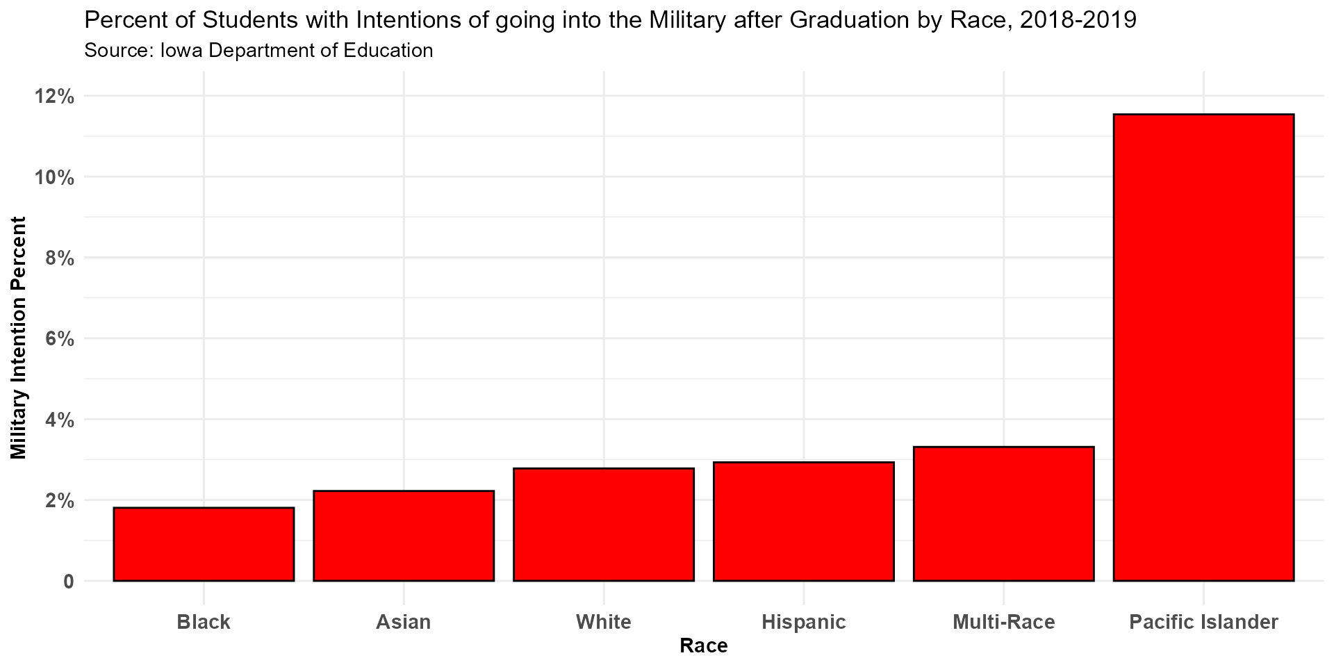
In the 2018-2019 school year, students who identify as black had the lowest military intention rates while students that identify as Pacific Islander had the highest military intention rate. Due to the small number of students that identify as Pacific Islander, this number may be inflated and it may be more difficult to make conclusive results from this the bottom-right graph alone.
Data
Sources:
Graduate Intentions by District: https://educateiowa.gov/document-type/graduate-intentions-district-including-graduate-counts
Graduate Intentions by Race and Gender 2008-2020: Data Request
Overall used for denominator in percents
overall <- ds %>%
  filter(Year != 2020,
         !(is.na(Count)),
         !(is.na(classification)),
         !(is.na(District.Name)),
         Intention %in% "Diploma Count") %>%
  mutate(Class = factor(ifelse(e2019 < 500,
                               "Under 500",
                               ifelse(e2019 >= 500 & e2019 < 2500,
                                      "500 - 2,499",
                                      ifelse(e2019 >= 2500 & e2019 < 10000,
                                             "2,500 - 9,999",
                                             ifelse(e2019 >= 10000 & e2019 < 25000,
                                                    "10,000 - 24,999",
                                                    "Over 25,000")))), levels = c(
                                                      "Over 25,000",
                                                      "10,000 - 24,999",
                                                      "2,500 - 9,999",
                                                      "500 - 2,499",
                                                      "Under 500"
                                                    ))) %>%
  group_by(Class, Year) %>%
  summarise(Overall = sum(Count))
Military to be used for numerator in percents
military <- ds %>%
  filter(Year != 2020,
         !(is.na(Count)),
         !(is.na(classification)),
         !(is.na(District.Name)),
         Intention %in% c("Military")) %>%
  mutate(Class = factor(ifelse(e2019 < 500,
                               "Under 500",
                               ifelse(e2019 >= 500 & e2019 < 2500,
                                      "500 - 2,499",
                                      ifelse(e2019 >= 2500 & e2019 < 10000,
                                             "2,500 - 9,999",
                                             ifelse(e2019 >= 10000 & e2019 < 25000,
                                                    "10,000 - 24,999",
                                                    "Over 25,000")))), levels = c(
                                                      "Over 25,000",
                                                      "10,000 - 24,999",
                                                      "2,500 - 9,999",
                                                      "500 - 2,499",
                                                      "Under 500"
                                                    ))) %>%
  group_by(Class, Year) %>%
summarise(Military = sum(Count))Creating military and overall for just 2019
military_2019 <- ds %>%
  filter(District.Name != "Glenwood",
         Year == 2019,
         Intention != "Diploma Count",
         Group == "Overall", # removing glenwood for same reason as above
         !(is.na(Count))) %>%
  group_by(Intention) %>%
  summarise(Count = sum(Count))

overall_2019 <- ds %>%
  filter(Year == 2019,
         District.Name != "Glenwood",
         Intention == "Diploma Count",
         Group == "Overall", # removing glenwood for same reason as above
         !(is.na(Count))) %>%
  group_by(Intention) %>%
  summarise(Count = sum(Count))

military_2019 <- military_2019 %>%
mutate(Rate = Count / overall_2019$Count * 100)Load in grad intentions and 2021 FRL data
grad_intents <- read_csv("../data_clean/dataClean_IAGradIntentions1920.csv")
#> Warning: Missing column names filled in: 'X1' [1]
frl_wide <- read_excel("../data_clean/2018-2019 FRL Data.xlsx", skip = 6)
Cleaning, joining, and formatting
##----filter-for-military-intentions------------------------------------------------------
military_data <- grad_intents %>%
  filter(Group == "Overall" & (Intention == "Military" | Intention == "Diploma Count"))
military_data <- military_data[,2:8]
military_wide <- spread(military_data, Intention, Count) %>%
  clean_names()
class(military_wide$district) = "numeric"

##----joining-military-and-FRL-data------------------------------------------------------
military_frl <- inner_join(frl_wide, military_wide, by = c("District" = "district"))
mil_frl_props <- military_frl %>%
  mutate(military_prop = military/diploma_count)
Methodology
Top left: Percent of High School Graduates with Military Intentions compared to Other Intentions after Graduation, 2019
military_2019 %>%
  ggplot(aes(x = reorder(Intention, Rate), y = Rate, fill = Intention)) +
  geom_col(color = "black") +
  theme_minimal() +
  labs(title = "Percent of High School Graduates with Military Intentions compared to Other Intentions after Graduation, 2019",
       subtitle = "Source: Iowa Department of Education") +
  scale_fill_manual(values = c("blue", "blue", "blue", "red", "blue", "blue", "blue", "blue", "blue")) +
  theme(legend.position = "none",
        axis.title = element_text(size = 11, face = "bold"),
        axis.text = element_text(size = 8, face = "bold")) +
  scale_y_continuous(breaks = c(0, 10, 20, 30, 40),
                     labels = c("0%", "10%", "20%", "30%", "40%"),
                     limits = c(0,40)) +
  xlab("Graduate Intention") +
  ylab("Intention Rate")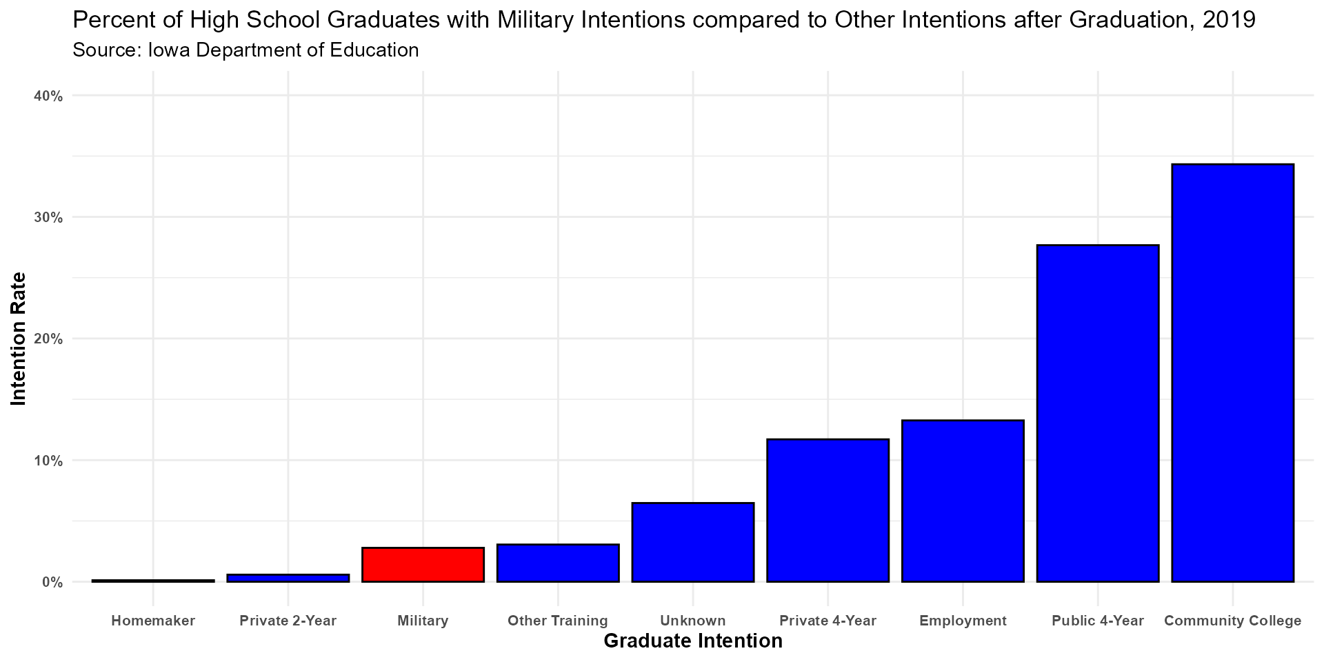
Top right: Percent of High School Graduates with Military Intentions after Graduation, 2010-2019
military %>%
  ggplot(aes(x = Year, y = Rate, color = Class)) +
  geom_line(size = 2) +
  scale_y_continuous(breaks = c(1, 1.5, 2, 2.5, 3, 3.5, 4, 4.5, 5),
                     labels = c("1%", "1.5%", "2%", "2.5%", "3%", "3.5%", "4%", "4.5%", "5%"),
                     limits = c(1, 5)) +
  scale_x_continuous(breaks = c(2010, 2011, 2012, 2013, 2014, 2015, 2016, 2017, 2018, 2019),
                     labels = c(2010, 2011, 2012, 2013, 2014, 2015, 2016, 2017, 2018, 2019)) +
  theme_minimal() +
  labs(title = "Percent of High School Graduates with Military Intentions after Graduation, 2010-2019",
       subtitle = "Source: Iowa Department of Education") +
  theme(axis.text = element_text(face = "bold", size = 11),
        axis.title = element_text(face = "bold", size = 11),
        axis.title.y = element_text(angle = 0, vjust = .5),
        legend.text = element_text(size = 11),
        legend.title = element_text(face = "bold", size = 11)) +
  scale_color_manual(name = "City Population", values =
                       c("#CA0020", "#F4A582", "light grey", "#92C5DE", "#0571B0"))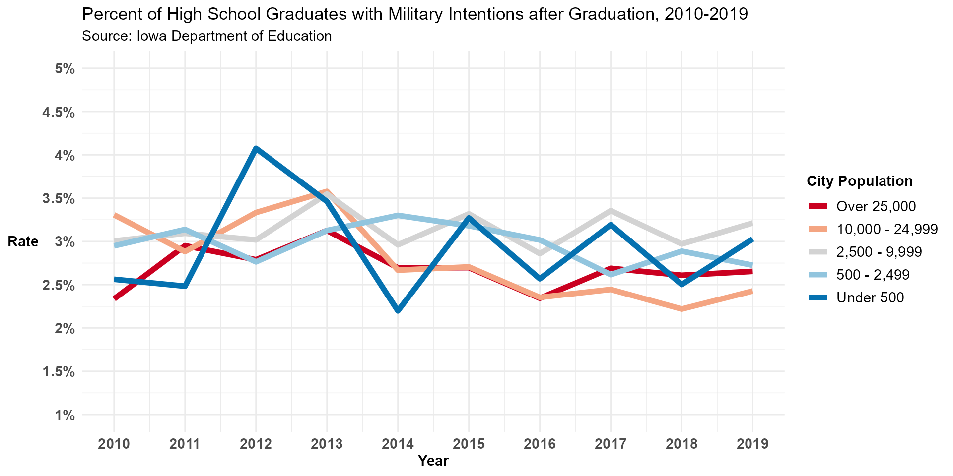
Bottom left: Iowa School Districts by Percent Military Intentions after Graduation and Percent Free/Reduced Lunch Eligibility, 2018-2019
military_scatter2 <- mil_frl_props %>%
  ggplot(aes(y = military_prop, x = `Free or Reduced Price Lunch`)) +
  geom_point() +
  labs(title = "Iowa School Districts by Free/Reduced Lunch Eligibility and Military Intent",
       subtitle = "Source: Department of Education",
       y = "Proportion of Military Intention",
       x = "Proportion Eligible for Free/Reduced Lunch") +
  theme_minimal()

military_scatter2
#> Warning: Removed 25 rows containing missing values (geom_point).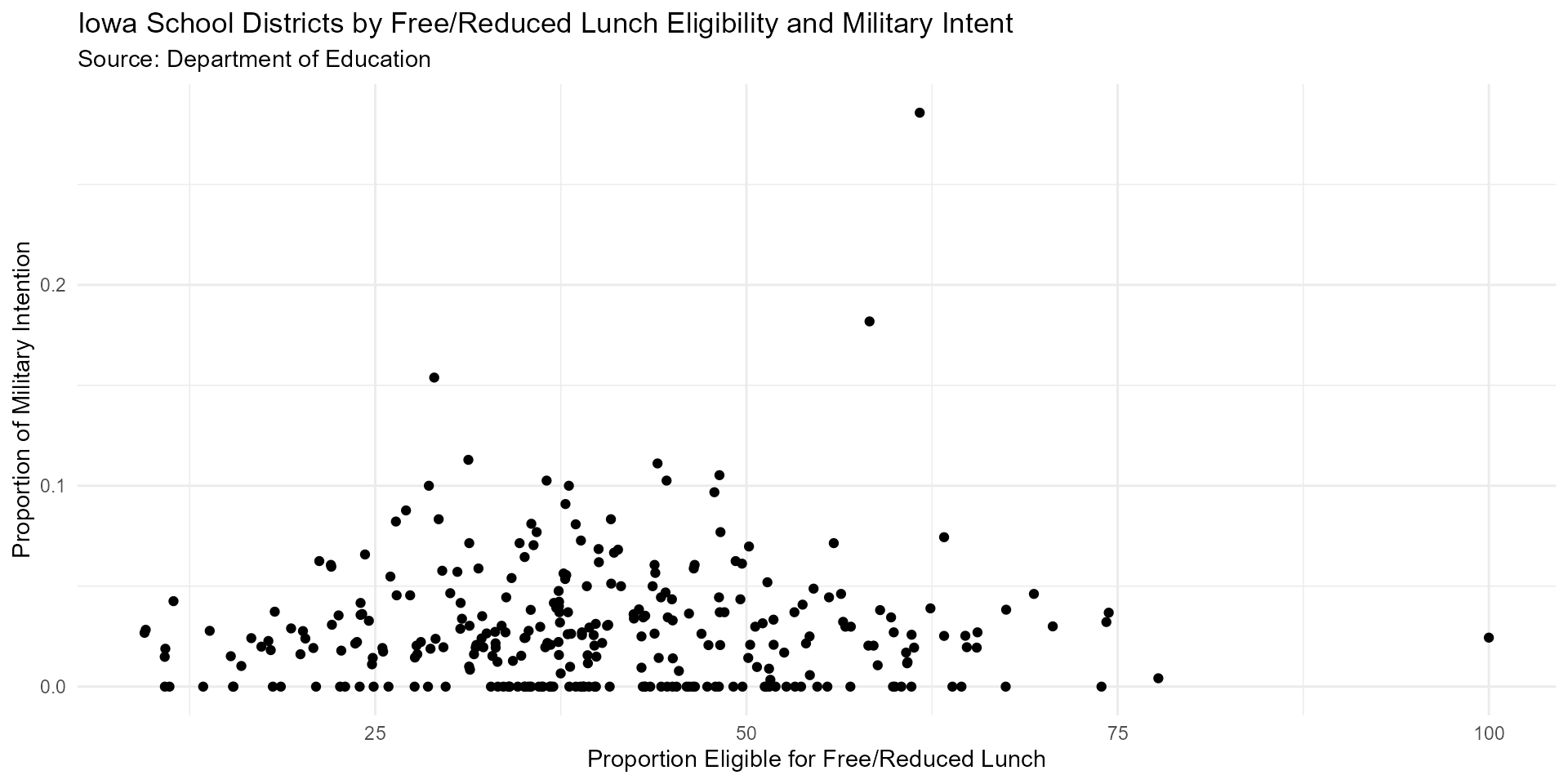
Bottom right: Percent of Students with Intentions of going into the Military after Graduation by Race, 2018-2019
ds %>%
  filter(Year == 2019,
         Intention == "Military",
         Group %in% c("White", "Black", "Hispanic", "Asian", "Pacific Islander", "Multi-Race")) %>%
  group_by(Group) %>%
  summarise(Count = sum(Count)) %>%
  left_join(overall_race, by = c("Group" = "Group")) %>%
  mutate(Rate = Count / Overall * 100) %>%
  ggplot(aes(x = reorder(Group, Rate), y = Rate)) +
  geom_col(color = "black", fill = "red") +
  theme_minimal() +
  labs(title = "Percent of Students with Intentions of going into the Military after Graduation by Race, 2018-2019",
       subtitle = "Source: Iowa Department of Education") +
  scale_y_continuous(breaks = c(0, 2, 4, 6, 8, 10, 12),
                     labels = c("0", "2%", "4%", "6%", "8%", "10%", "12%"),
                     limits = c(0,12)) +
  xlab("Race") +
  ylab("Military Intention Percent") +
  theme(axis.title = element_text(size = 11, face = "bold"),
        axis.text = element_text(size = 11, face = "bold"))