Which Groups Vary in Educational Attainment in Iowa?
EduAttainment_poster.RmdIn this article, we explore which groups, communities, and areas in Iowa are under-served and underachieving in educational attainment.
Findings
Educational attainment varies between males and females among degree levels. Most notably, males are obtaining more Professional and Doctorates degrees while females are obtaining more Bachelor's and Master's degrees in Iowa.
Median earnings across all degree levels show females earning less than men in all levels of educational attainment.
Differences in levels of educational attainment differ further between race groups than between sexes.
Educational attainment shows Asian having the highest proportion of Bachelor's degrees and higher, while Latino has the highest frequency of achieving less than a high school diploma.
Data
Loading, joining, and cleaning data
##----load-in-packages--------------------------------------------------------------
library(tidycensus)
#> Warning: package 'tidycensus' was built under R version 4.0.5
library(tidyverse)
#> Warning: package 'tidyverse' was built under R version 4.0.3
#> Warning: package 'ggplot2' was built under R version 4.0.5
#> Warning: package 'tibble' was built under R version 4.0.3
#> Warning: package 'tidyr' was built under R version 4.0.3
#> Warning: package 'readr' was built under R version 4.0.3
#> Warning: package 'purrr' was built under R version 4.0.3
#> Warning: package 'dplyr' was built under R version 4.0.3
library(tigris)
#> Warning: package 'tigris' was built under R version 4.0.5
library(mapview)
#> Warning: package 'mapview' was built under R version 4.0.5
library(leafsync)
#> Warning: package 'leafsync' was built under R version 4.0.5
library(leaflet)
#> Warning: package 'leaflet' was built under R version 4.0.5
library(plotly)
#> Warning: package 'plotly' was built under R version 4.0.4
library(spdep)
#> Warning: package 'spdep' was built under R version 4.0.5
#> Warning: package 'sp' was built under R version 4.0.5
#> Warning: package 'spData' was built under R version 4.0.5
#> Warning: package 'sf' was built under R version 4.0.5
library(tmap)
#> Warning: package 'tmap' was built under R version 4.0.5
library(tmaptools)
#> Warning: package 'tmaptools' was built under R version 4.0.5
library(remotes)
#> Warning: package 'remotes' was built under R version 4.0.5
library(crsuggest)
#> Warning: package 'crsuggest' was built under R version 4.0.5
library(ggplot2)
library(tigris)
library(dplyr)
library(forcats)
library(sf)
library(viridis)
#> Warning: package 'viridis' was built under R version 4.0.5
#> Warning: package 'viridisLite' was built under R version 4.0.5
library(viridisLite)
library(stringr)
library(xfun)
#> Warning: package 'xfun' was built under R version 4.0.5
options(tigris_use_cache = TRUE)

##----iowa-sex-edu-data-----------------------------------------------------------
iowa <- get_acs(
  state = "IA",
  geography = "state",
  variables = c(M_no_schooling1 = "B15002_003",
                M_no_schooling2 = "B15002_004",
                M_no_schooling3 = "B15002_005",
                M_no_schooling4 = "B15002_006",
                M_no_schooling5 = "B15002_007",
                M_no_schooling6 = "B15002_008",
                M_no_schooling7 = "B15002_009",
                M_no_schooling8 = "B15002_010",
                M_highschool_diploma = "B15002_011",
                M_some_college1 = "B15002_012",
                M_some_college2 = "B15002_013",
                M_associates = "B15002_014",
                M_bachelors = "B15002_015",
                M_masters = "B15002_016",
                M_professional = "B15002_017",
                M_doctorate = "B15002_018",
                F_no_schooling1 = "B15002_020",
                F_no_schooling2 = "B15002_021",
                F_no_schooling3 = "B15002_022",
                F_no_schooling4 = "B15002_023",
                F_no_schooling5 = "B15002_024",
                F_no_schooling6 = "B15002_025",
                F_no_schooling7 = "B15002_026",
                F_no_schooling8 = "B15002_027",
                F_highschool_diploma = "B15002_028",
                F_some_college1 = "B15002_029",
                F_some_college2 = "B15002_030",
                F_associates = "B15002_031",
                F_bachelors = "B15002_032",
                F_masters = "B15002_033",
                F_professional = "B15002_034",
                F_doctorate = "B15002_035")
)

iowa

#--another way, cleaner
iowa_filtered <- iowa %>%
  mutate(var2 = str_remove(variable, "[:digit:]")) %>%
  group_by(GEOID, NAME, var2) %>%
  summarise(estimate = sum(estimate),
            moe = moe_sum(estimate, moe))

iowa_best <- iowa_filtered %>%
  mutate(SEX = str_sub(var2, 1, 1))

iowa_final <- iowa_best %>%
  mutate(estimate = ifelse(SEX == "M", -estimate, estimate),
         education = str_sub(var2,3,-1))


##----renaming-education-categories-----------------------------------------------
iowa_final <- iowa_final %>%
  mutate(category = ifelse(iowa_final$education == "no_schooling", "Less Than High School",
                           ifelse(iowa_final$education == "highschool_diploma", "High School Diploma",
                                  ifelse(iowa_final$education == "some_college", "Some College",
                                         ifelse(iowa_final$education == "associates", "Associates",
                                                ifelse(iowa_final$education == "bachelors", "Bachelors",
                                                       ifelse(iowa_final$education == "masters", "Masters",
                                                              ifelse(iowa_final$education == "professional", "Professional", "Doctorate"))))))),
         sex_full = ifelse(iowa_final$SEX == "F", "Female", "Male"))

##----all-attainment-variables-by-race-----------------------------------------------
attain_vars <- c(M_Less_Than_High_School_White = "C15002A_003",
                 M_High_School_Diploma_White = "C15002A_004",
                 M_Some_College_White = "C15002A_005",
                 M_Bachelors_Degree_White = "C15002A_006",
                 F_Less_Than_High_School_White = "C15002A_008",
                 F_High_School_Diploma_White = "C15002A_009",
                 F_Some_College_White = "C15002A_010",
                 F_Bachelors_Degree_White = "C15002A_011",
                 M_Less_Than_High_School_Black = "C15002B_003",
                 M_High_School_Diploma_Black = "C15002B_004",
                 M_Some_College_Black = "C15002B_005",
                 M_Bachelors_Degree_Black = "C15002B_006",
                 F_Less_Than_High_School_Black = "C15002B_008",
                 F_High_School_Diploma_Black = "C15002B_009",
                 F_Some_College_Black = "C15002B_010",
                 F_Bachelors_Degree_Black = "C15002B_011",
                 M_Less_Than_High_School_Asian = "C15002D_003",
                 M_High_School_Diploma_Asian = "C15002D_004",
                 M_Some_College_Asian = "C15002D_005",
                 M_Bachelors_Degree_Asian = "C15002D_006",
                 F_Less_Than_High_School_Asian = "C15002D_008",
                 F_High_School_Diploma_Asian = "C15002D_009",
                 F_Some_College_Asian = "C15002D_010",
                 F_Bachelors_Degree_Asian = "C15002D_011",
                 M_Less_Than_High_School_Latin = "C15002I_003",
                 M_High_School_Diploma_Latin = "C15002I_004",
                 M_Some_College_Latin = "C15002I_005",
                 M_Bachelors_Degree_Latin = "C15002I_006",
                 F_Less_Than_High_School_Latin = "C15002I_008",
                 F_High_School_Diploma_Latin = "C15002I_009",
                 F_Some_College_Latin = "C15002I_010",
                 F_Bachelors_Degree_Latin = "C15002I_011")
##----attainment-vars-by-sex-and-race------------------------------------------------
white_male <- c(M_Less_Than_High_School_White = "C15002A_003",
             M_High_School_Diploma_White = "C15002A_004",
             M_Some_College_White = "C15002A_005",
             M_Bachelors_Degree_White = "C15002A_006")

white_female <- c(F_Less_Than_High_School_White = "C15002A_008",
                  F_High_School_Diploma_White = "C15002A_009",
                  F_Some_College_White = "C15002A_010",
                  F_Bachelors_Degree_White = "C15002A_011")

black_male <- c(M_Less_Than_High_School_Black = "C15002B_003",
           M_High_School_Diploma_Black = "C15002B_004",
           M_Some_College_Black = "C15002B_005",
           M_Bachelors_Degree_Black = "C15002B_006")

black_female <- c(F_Less_Than_High_School_Black = "C15002B_008",
                  F_High_School_Diploma_Black = "C15002B_009",
                  F_Some_College_Black = "C15002B_010",
                  F_Bachelors_Degree_Black = "C15002B_011")

asian_male <- c(M_Less_Than_High_School_Asian = "C15002D_003",
           M_High_School_Diploma_Asian = "C15002D_004",
           M_Some_College_Asian = "C15002D_005",
           M_Bachelors_Degree_Asian = "C15002D_006")

asian_female <- c(F_Less_Than_High_School_Asian = "C15002D_008",
                  F_High_School_Diploma_Asian = "C15002D_009",
                  F_Some_College_Asian = "C15002D_010",
                  F_Bachelors_Degree_Asian = "C15002D_011")

latino_male <- c(M_Less_Than_High_School_Latin = "C15002I_003",
            M_High_School_Diploma_Latin = "C15002I_004",
            M_Some_College_Latin = "C15002I_005",
            M_Bachelors_Degree_Latin = "C15002I_006")

latino_female <- c(F_Less_Than_High_School_Latin = "C15002I_008",
                   F_High_School_Diploma_Latin = "C15002I_009",
                   F_Some_College_Latin = "C15002I_010",
                   F_Bachelors_Degree_Latin = "C15002I_011")

##----getting-data-by-race-and-sex--------------------------------------------------
white_male_data <- get_acs(
  geography = "state",
  state = "IA",
  variables = white_male,
  summary_var = "C15002A_002"
)


white_female_data <- get_acs(
  geography = "state",
  state = "IA",
  variables = white_female,
  summary_var = "C15002A_007"
)

black_male_data <- get_acs(
  geography = "state",
  state = "IA",
  variables = black_male,
  summary_var = "C15002B_002"
)

black_female_data <- get_acs(
  geography = "state",
  state = "IA",
  variables = black_female,
  summary_var = "C15002B_007"
)

asian_male_data <- get_acs(
  geography = "state",
  state = "IA",
  variables = asian_male,
  summary_var = "C15002D_002"
)

asian_female_data <- get_acs(
  geography = "state",
  state = "IA",
  variables = asian_female,
  summary_var = "C15002D_007"
)

latino_male_data <- get_acs(
  geography = "state",
  state = "IA",
  variables = latino_male,
  summary_var = "C15002I_002"
)

latino_female_data <- get_acs(
  geography = "state",
  state = "IA",
  variables = latino_female,
  summary_var = "C15002I_007"
)

##----calculating-percent-of-each-race/sex's-educational-attainment-----------------
white_male_pct <- white_male_data %>%
  mutate(edu_pct = estimate/summary_est * 100)

white_female_pct <- white_female_data %>%
  mutate(edu_pct = estimate/summary_est * 100)

black_male_pct <- black_male_data %>%
  mutate(edu_pct = estimate/summary_est * 100)

black_female_pct <- black_female_data %>%
  mutate(edu_pct = estimate/summary_est * 100)

asian_male_pct <- asian_male_data %>%
  mutate(edu_pct = estimate/summary_est * 100)

asian_female_pct <- asian_female_data %>%
  mutate(edu_pct = estimate/summary_est * 100)

latino_male_pct <- latino_male_data %>%
  mutate(edu_pct = estimate/summary_est * 100)

latino_female_pct <- latino_female_data %>%
  mutate(edu_pct = estimate/summary_est * 100)

##----merging-all-the-race-&-sex-data-together-------------------------------------

white_pct <- rbind(white_male_pct, white_female_pct)

black_pct <- rbind(black_male_pct, black_female_pct)

asian_pct <- rbind(asian_male_pct, asian_female_pct)

latino_pct <- rbind(latino_male_pct, latino_female_pct)

white_black_pct <- rbind(white_pct, black_pct)

asian_latino_pct <- rbind(asian_pct, latino_pct)

all_race_sex_data <- rbind(white_black_pct, asian_latino_pct)

##----filtering-the-data------------------------------------------------------------------------

all_data_filtered <- all_race_sex_data %>%
  mutate(education = str_sub(variable,3,-7),
         SEX = str_sub(variable,1,1),
         race = str_sub(variable,-5,-1))

all_data_complete <- all_data_filtered %>%
  mutate(estimate = ifelse(SEX == "M", -estimate, estimate))

##----graph-the-completed-race/sex-data--------------------------------------------------------
all_data_complete$education = factor(all_data_complete$education, levels = c("Less_Than_High_School", "High_School_Diploma",
                                                             "Some_College", "Bachelors_Degree"),
                             labels = c("Less than High School",
                                        "High School Diploma",
                                        "Some College",
                                        "Bachelors Degree or Higher"))

all_data_complete$race = factor(all_data_complete$race, levels = c("White", "Black",
                                                                             "Asian", "Latin"),
                                     labels = c("White",
                                                "Black",
                                                "Asian",
                                                "Latino"))
##----by-race-AND-gender---------------------------------------------------------------------
both_data <- all_data_filtered %>%
  mutate(edu_pct = ifelse(SEX == "M", -edu_pct, edu_pct))

both_data$education = factor(both_data$education, levels = c("Less_Than_High_School", "High_School_Diploma",
                                                             "Some_College", "Bachelors_Degree"),
                       labels = c("Less than High School",
                                  "High School Diploma or GED",
                                  "Some College",
                                  "Bachelors Degree or Higher"))
both_data$race = factor(both_data$race, levels = c("White", "Black",
                                                        "Asian", "Latin"),
                        labels = c("White",
                                   "Black",
                                   "Asian",
                                   "Latino"))

#Datat ACS B28006 Educational attainment and computer and type of internet in the home
iacomp_ed <-  get_acs(
  geography = "county",
  state = "IA",
  variables = c(

    #less than high school
    #less_than_hs = "B28006_002",
    lessthanhs_computer = "B28006_003",
    lessthanhs_dialup = "B28006_004",
    lessthanhs_broadband = "B28006_005",
    lessthanhs_wointernet = "B28006_006",
    lessthanhs_nocomputer = "B28006_007",

    #high school, some college, or associates degree
    #hs_or_some_coll = "B28006_008",
    hsorsomecoll_computer = "B28006_009",
    hsorsomecoll_dialup = "B28006_010",
    hsorsomecoll_broadband = "B28006_011",
    hsorsomecoll_wointernet = "B28006_012",
    hsorsomecoll_nocomputer = "B28006_013",

    #bachelors degree or more schooling
    #bach_or_more = "B28006_014",
    bachormore_computer = "B28006_015",
    bachormore_dialup = "B28006_016",
    bachormore_broadband = "B28006_017",
    bachormore_wointernet = "B28006_018",
    bachormore_nocomputer = "B28006_019"),


  summary_var = "B28006_001",

  survey = "acs5",
  geometry = TRUE

) %>%
  mutate(percent = 100 * (estimate / summary_est))


head(iacomp_ed)

#military ed att data

vet_edatt_level <- get_acs(
  geography = "county",
  state = "IA",
  variables = c(High_School = "B21003_003",
                High_School_or_GED = "B21003_004",
                Some_College_or_Associates = "B21003_005",
                Bachelors_Degree_or_More = "B21003_006"),
  summary_var = "B21003_002",
  geometry = TRUE
) %>%
  mutate(percent = 100 * (estimate / summary_est))

#setting up spatial
ia_counties <- counties("IA", cb = TRUE)
st_crs(ia_counties)
#
ia_crs <- suggest_crs(ia_counties)
glimpse(ia_crs)
#
ia_projected <- st_transform(ia_counties, crs = 6463)
head(ia_projected)

#B15010 Area of first bachelors degree

iaacs_edatt <-  get_acs(
  geography = "county",
  state = "IA",
  variables = c(

    #first 4yr degree
    co_ma_st = "B15010_002",
    bio_ag_en = "B15010_003",
    phys_sci = "B15010_004",
    psych_sci = "B15010_005",
    soc_sci = "B15010_006",
    engine = "B15010_007",
    multi = "B15010_008",
    sci_efi = "B15010_009",
    busi = "B15010_010",
    educ = "B15010_011",
    lit_lang = "B15010_012",
    hist_l_a = "B15010_013",
    vis_arts = "B15010_014",
    comm = "B15010_015",
    art_hum_ot = "B15010_016"
  ),


  summary_var = "B15010_001",

  survey = "acs1",
  geometry = TRUE

) %>%
  mutate(percent = 100 * (estimate / summary_est)

  )


glimpse(iaacs_edatt)

head(iaacs_edatt)

#Cleaning 1st batch data
ia_first_bach <- filter(iaacs_edatt,
                        variable == "co_ma_st" |
                          variable == "bio_ag_en" |
                          variable == "phys_sci" |
                          variable == "psych_sci" |
                          variable == "soc_sci" |
                          variable == "engine" |
                          variable == "multi" |
                          variable == "sci_efi" |
                          variable == "busi" |
                          variable == "educ" |
                          variable == "lit_lang" |
                          variable == "hist_l_a" |
                          variable == "vis_arts" |
                          variable == "comm" |
                          variable == "art_hum_ot")


head(ia_first_bach)

str(ia_first_bach$variable)


ia_first_bach$variable <- factor(ia_first_bach$variable,
                                 levels = c("co_ma_st",
                                            "bio_ag_en",
                                            "phys_sci",
                                            "psych_sci",
                                            "soc_sci",
                                            "engine",
                                            "multi",
                                            "sci_efi",
                                            "busi",
                                            "educ",
                                            "lit_lang",
                                            "hist_l_a",
                                            "vis_arts",
                                            "comm",
                                            "art_hum_ot"),
                                 labels = c("Comp Sci, Math, or Stat",
                                            "Bio, Ag, or Env Sci",
                                            "Physical Sci",
                                            "Psychology",
                                            "Social Science",
                                            "Engineering",
                                            "Multi-Discipline",
                                            "Science & Engineering Related",
                                            "Business",
                                            "Education",
                                            "Lit & Lang",
                                            "Lib Arts & History",
                                            "Visual, Perfomace Art",
                                            "Communication",
                                            "Arts, Humanities, and Other"
                                 ))


ia_first_bach$variable <- fct_explicit_na(ia_first_bach$variable)

str(ia_first_bach)

str(ia_first_bach$variable)

levels(ia_first_bach$variable)

fct_count(ia_first_bach$variable)
Methodology
Educational Attainment by Sex Pyramid Graph
pyramid_plot <- iowa_final %>% mutate(category = fct_relevel(category, "Less Than High School", "High School Diploma",
                                                                      "Some College", "Associates", "Bachelors",
                                                                      "Masters", "Professional", "Doctorate")) %>%
  ggplot( aes(x = estimate, y = category, fill = sex_full)) +
  geom_col() +
  scale_x_continuous(labels = function(y) paste0(abs(y / 1000), "k")) +
  labs(title = "Educational Attainment of Adults Age 25 and Over by Sex in Iowa",
       x = "",
       y = "",
       caption = "Source: 2019 ACS Data",
       fill = "") +
  geom_vline(xintercept = 0) +
  scale_fill_manual(values = c("#D81E3F", "#2A6EBB")) +
  theme_minimal()

pyramid_plot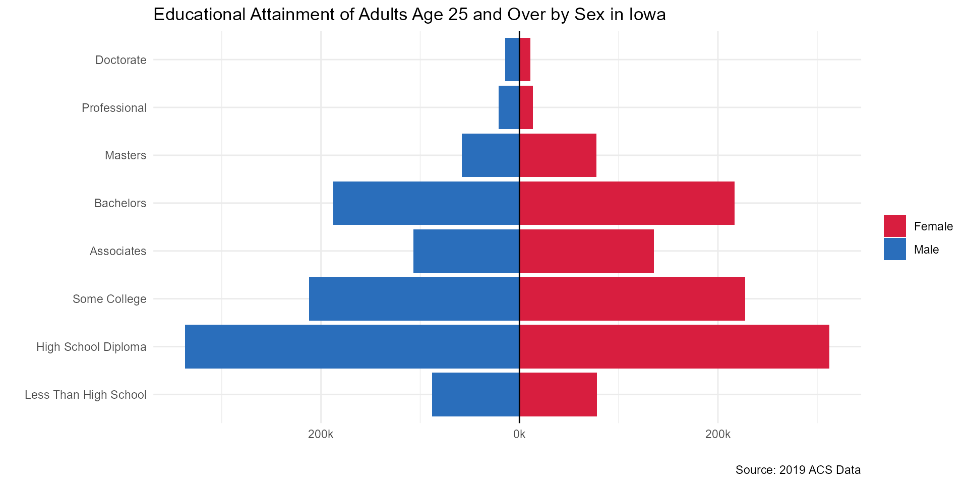
Educational Attainment by Race Bar Graph
race_sex_graph <- all_data_complete %>%
  mutate(education = fct_relevel(education, "Less_Than_High_School", "High_School_Diploma",
                                 "Some_College", "Bachelors_Degree")) %>%
  ggplot(aes(x = race, y = edu_pct, fill = education)) +
  geom_bar(position = "dodge", stat = "identity") +
  labs(title = "Educational Attainment in Adults Age 25 and Over by Race in Iowa",
       x = "",
       y = "Percentage of Educational Attainment",
       subtitle = "Source: 2015-2019 ACS Data",
       fill = "Education") +
  scale_fill_manual(values = c("#ca0020","#f4a582","#92c5de","#0571b0")) +
  theme_minimal()
#> Warning: Problem with `mutate()` input `education`.
#> i Unknown levels in `f`: Less_Than_High_School, High_School_Diploma, Some_College, Bachelors_Degree
#> i Input `education` is `fct_relevel(...)`.
#> Warning: Unknown levels in `f`: Less_Than_High_School, High_School_Diploma,
#> Some_College, Bachelors_Degree

race_sex_graph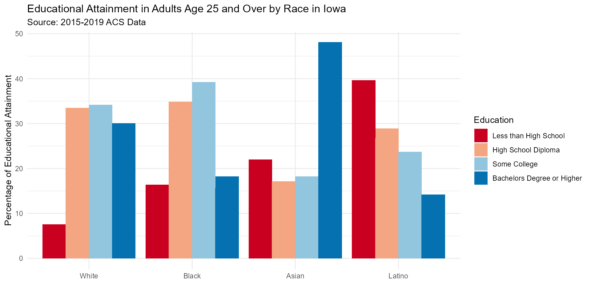
Educational Attainment by Race and Sex Pyramid Graph
both_data_graph <- both_data %>%
  ggplot() +
  geom_col(aes(x = edu_pct, y = education, fill = race), position = "dodge", stat = "identity", color = "black") +
  theme_minimal() +
  labs(title = "Educational Attainment by Race & Gender in Iowa",
       x = "Proportion of Educational Attainment",
       y = "",
       subtitle = "Source: 2015-2019 ACS Data",
       fill = "Race") +
  geom_label(aes(x = -30, y = 4.4), label = "Male") +
  geom_label(aes(x = 30, y = 4.4), label = "Female") +
  geom_vline(xintercept = 0) +
  scale_fill_manual(values = c("#ca0020","#f4a582","#92c5de","#0571b0"))
#> Warning: Ignoring unknown parameters: stat

both_data_graph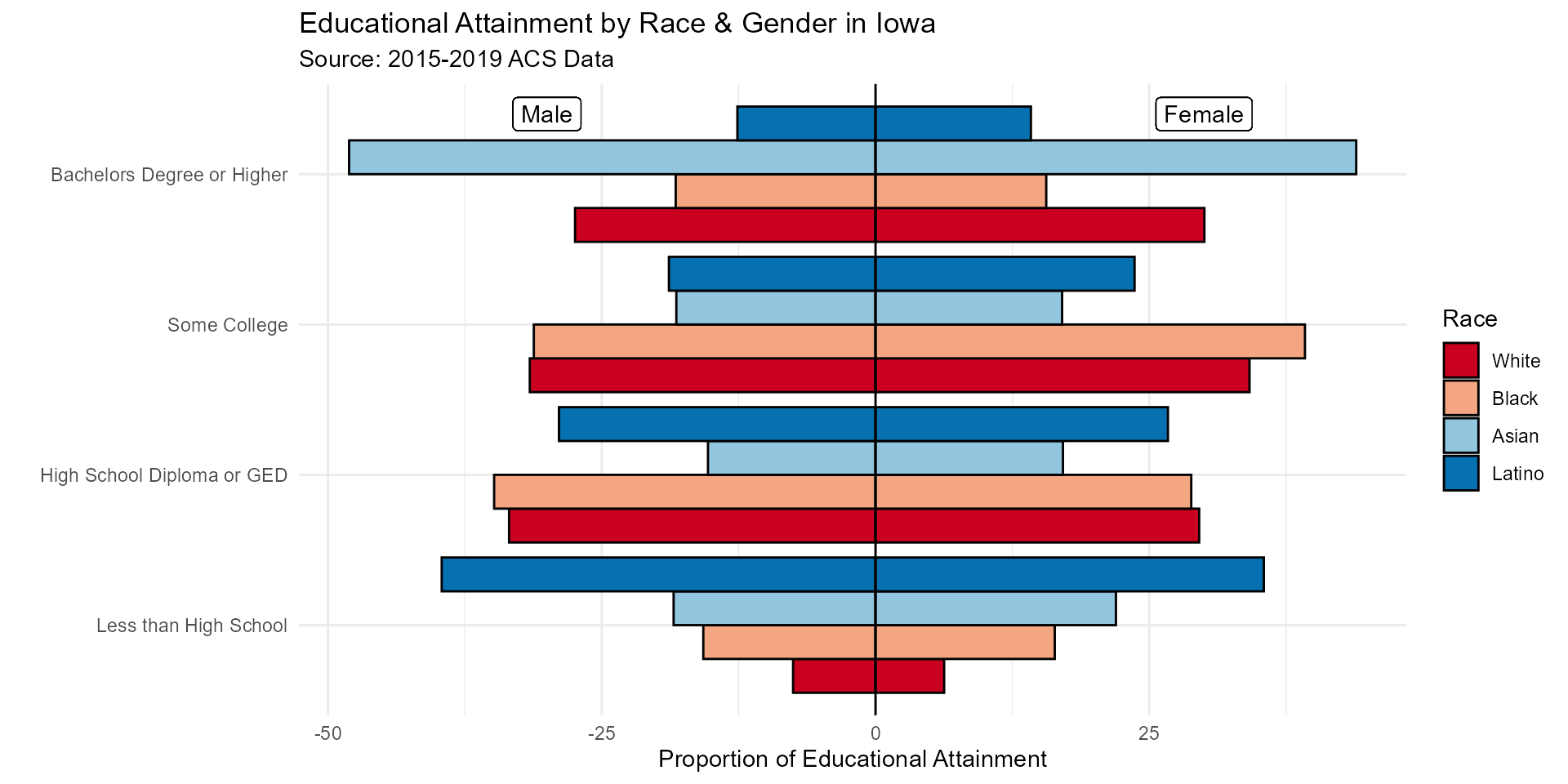
Proportion of Population with Bachelor's Degree Iowa Map
iavb_pplot <- filter(vet_edatt_level ,
                       variable == "Bachelors_Degree_or_More")

bach_ve <- tm_shape(iavb_pplot) +
  tm_layout(main.title = "Percent by County of Veterans Iowans\nwith A Bachelors Degree or Higher", main.title.size = 1.25, main.title.position = "center", legend.outside = TRUE, frame = FALSE) +
  tm_polygons(col = "percent", alpha = 0.5,
              palette = c("#C41230", "white","#005DAB" ), style = "jenks", n = 5)

bach_ve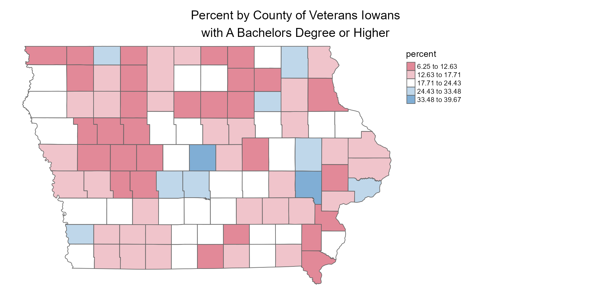
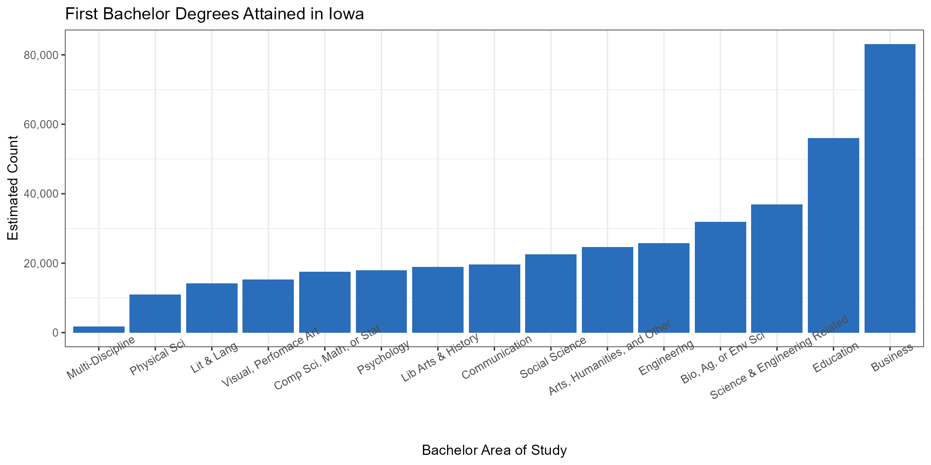
Bachelor's Degrees by Type Bar Graph
ia_bach_plot <- ggplot(ia_first_bach,
                       aes(x = reorder(variable, estimate), y = estimate)) +
                geom_col(fill = "#2A6EBB") +
                ggtitle("First Bachelor Degrees Attained in Iowa") +
                labs(x = "Bachelor Area of Study", y = "Estimated Count") +
                theme_bw() +
  scale_y_continuous(labels = scales::comma) +
  theme(panel.grid.major.y = element_blank(),
        axis.text.x = element_text(angle = 30))


ia_bach_plot