Which Students Have Intentions of Going to College After Graduation?

Findings

• In the 2020-2021 school year, female students had a much higher college intention percent than male students.

• In the same school year, students that identified as Pacific Islander, Hispanic, Black, and Multi-Race had college intention rates at lower rates than students that identified as White or Asian.

• College Intention Rates varied from 25% all the way to 80% across districts in Iowa for the 2018-2019 school year. Such variation is possibly due to different school sizes, rural/urban status, or other factors.

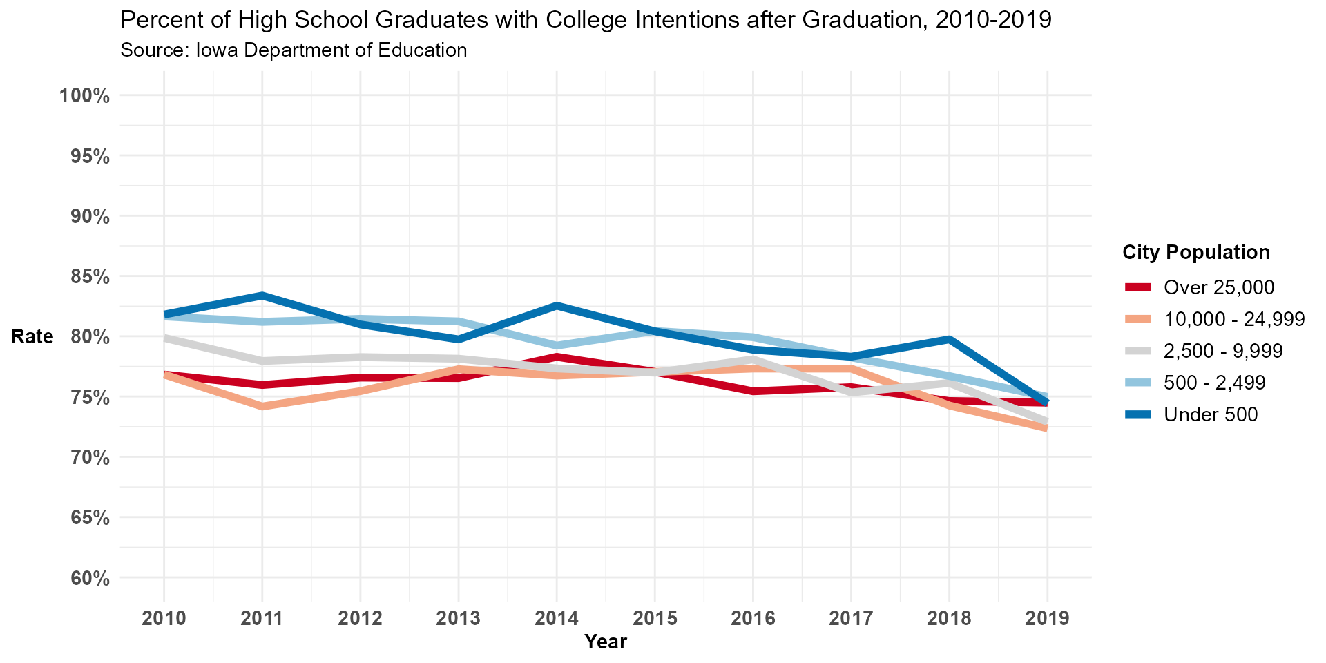
• Since 2010, the college intention rate has significantly dropped for all districts regardless of city population.

Data

Sources:

• Graduate Intentions by District: https://educateiowa.gov/document-type/graduate-intentions-district-including-graduate-counts

• Graduate Intentions by Race and Gender 2008-2020: Data Request

Loading in fist dataset and removing all non-responses from dataset due to COVID-19 impacting the survey

ds <- na.omit(read.csv("../data_clean/dataClean_IAGradIntentions1920.csv"))

ds_overall <- ds %>%
  filter(Group %in% "Overall",
         Intention %in% "Diploma Count") %>%
  group_by(Group) %>%
  summarise(Graduates = sum(Count))

ds_noresponse <- ds %>%
  filter(Group %in% "Overall",
         Intention %in% "No Graduate Intentions Reported") %>%
  group_by(Group) %>%
  summarise(`No Responses` = sum(Count))

total_responses <- ds_overall$Graduates - ds_noresponse$`No Responses`

ds_male <- ds %>%
  filter(Group %in% "Male",
         Intention %in% "Diploma Count") %>%
  group_by(Group) %>%
  summarise(Graduates = sum(Count))

ds_male_noresponse <- ds %>%
  filter(Group %in% "Male",
         Intention %in% "No Graduate Intentions Reported") %>%
  group_by(Group) %>%
  summarise(`No Responses` = sum(Count))

male_responses <- ds_male$Graduates - ds_male_noresponse$`No Responses`

female_responses <- total_responses - male_responses

Removing non-responses from race groups

### White
ds_white <- ds %>%
  filter(Group %in% "White",
         Intention %in% "Diploma Count") %>%
  group_by(Group) %>%
  summarise(Graduates = sum(Count))

ds_white_noresponse <- ds %>%
  filter(Group %in% "White",
         Intention %in% "No Graduate Intentions Reported") %>%
  group_by(Group) %>%
  summarise(`No Responses` = sum(Count))

white_responses <- ds_white$Graduates - ds_white_noresponse$`No Responses`


### Black
ds_black <- ds %>%
  filter(Group %in% "Black",
         Intention %in% "Diploma Count") %>%
  group_by(Group) %>%
  summarise(Graduates = sum(Count))

ds_black_noresponse <- ds %>%
  filter(Group %in% "Black",
         Intention %in% "No Graduate Intentions Reported") %>%
  group_by(Group) %>%
  summarise(`No Responses` = sum(Count))

black_responses <- ds_black$Graduates - ds_black_noresponse$`No Responses`


### Hispanic
ds_hispanic <- ds %>%
  filter(Group %in% "Hispanic",
         Intention %in% "Diploma Count") %>%
  group_by(Group) %>%
  summarise(Graduates = sum(Count))

ds_hispanic_noresponse <- ds %>%
  filter(Group %in% "Hispanic",
         Intention %in% "No Graduate Intentions Reported") %>%
  group_by(Group) %>%
  summarise(`No Responses` = sum(Count))

hispanic_responses <- ds_hispanic$Graduates - ds_hispanic_noresponse$`No Responses`


### Asian
ds_asian <- ds %>%
  filter(Group %in% "Asian",
         Intention %in% "Diploma Count") %>%
  group_by(Group) %>%
  summarise(Graduates = sum(Count))

ds_asian_noresponse <- ds %>%
  filter(Group %in% "Asian",
         Intention %in% "No Graduate Intentions Reported") %>%
  group_by(Group) %>%
  summarise(`No Responses` = sum(Count))

asian_responses <- ds_asian$Graduates - ds_asian_noresponse$`No Responses`


### Pacific Islander
ds_pi <- ds %>%
  filter(Group %in% "Pacific Islander",
         Intention %in% "Diploma Count") %>%
  group_by(Group) %>%
  summarise(Graduates = sum(Count))

ds_pi_noresponse <- ds %>%
  filter(Group %in% "Pacific Islander",
         Intention %in% "No Graduate Intentions Reported") %>%
  group_by(Group) %>%
  summarise(`No Responses` = sum(Count))

pi_responses <- ds_pi$Graduates - ds_pi_noresponse$`No Responses`


### Multi-Race
ds_multi <- ds %>%
  filter(Group %in% "Multi-Race",
         Intention %in% "Diploma Count") %>%
  group_by(Group) %>%
  summarise(Graduates = sum(Count))

ds_multi_noresponse <- ds %>%
  filter(Group %in% "Multi-Race",
         Intention %in% "No Graduate Intentions Reported") %>%
  group_by(Group) %>%
  summarise(`No Responses` = sum(Count))

multi_responses <- ds_multi$Graduates - ds_multi_noresponse$`No Responses`

Loading in new datasets and cleaning

ds2 <- na.omit(read.csv("../data_clean/dataClean_IAGradIntentions09-20.csv"))
ds2$classification <- factor(ds2$classification)
ds2$District.Name <- factor(ds2$District.Name)

ds2_2019 <- ds2 %>%
  filter(Year == 2019,
         Intention == "Diploma Count",
         Group == "Overall") %>%
  group_by(District) %>%
  summarise(District = District.Name,
            Graduates = sum(Count),
            Group = classification,
            GEOID = UNIFIED) %>%
  distinct()

schools <- school_districts("Iowa", year = 2020, progress_bar = F)

## standarzing district names
schools <- schools %>%
  mutate(GEOID = str_sub(GEOID, 3),
         GEOID = as.numeric(GEOID))

schools <- schools %>%
  left_join(ds2_2019, by = ("GEOID" = "GEOID")) %>%
  select(1:15, Group, Graduates)

schools$Group[is.na(schools$Group)] <- "Rural"

schools$Group <- factor(schools$Group, levels = c("Rural",
                                                  "Rural Plus",
                                                  "Urban Cluster",
                                                  "Micropolitan",
                                                  "Micro/Metro",
                                                  "Metropolitan"))

dist_coll <- ds2 %>%
  filter(Year == 2019,
         Intention %in% c("Private 4-Year", "Public 4-Year", "Community College", "Private 2-Year"),
         Group == "Overall") %>%
         group_by(District) %>%
         summarise(District = District.Name,
                   College = sum(Count)) %>%
  distinct()

schools <- schools %>%
  left_join(dist_coll, by = c("District" = "District")) %>%
  mutate(`College Rate` = College / Graduates * 100)

## Throwing out Glenwood School District as 167/171 graduates reported "Other" as their ds2ion.
schools$`College Rate`[schools$District == "Glenwood"] <- NA

## Binning districts into four groups
schools <- schools %>%
  mutate(CR.Bins = factor(ifelse(`College Rate` < 50, 
                          "25%-49%",
                          ifelse(`College Rate` >= 50 & `College Rate` < 65, 
                                 "50%-64%",
                                 ifelse(`College Rate` >= 65 & `College Rate` < 80,
                                        "65%-79%",
                                        "80+%")))))

Cleaning and formatting data

college <- ds2 %>%
  filter(Year != 2020,
         !(is.na(Count)),
         !(is.na(classification)),
         !(is.na(District.Name)),
         Intention %in% c("Private 4-Year", "Public 4-Year", "Community College", "Private 2-Year")) %>%
  mutate(Class = factor(ifelse(e2019 < 500, 
                                 "Under 500",
                                 ifelse(e2019 >= 500 & e2019 < 2500, 
                                        "500 - 2,499",
                                        ifelse(e2019 >= 2500 & e2019 < 10000,
                                               "2,500 - 9,999",
                                               ifelse(e2019 >= 10000 & e2019 < 25000,
                                                      "10,000 - 24,999",
                                                      "Over 25,000")))), levels = c(
                                                        "Over 25,000",
                                                        "10,000 - 24,999",
                                                        "2,500 - 9,999",
                                                        "500 - 2,499",
                                                        "Under 500"
                                                      ))) %>%
  group_by(Class, Year) %>%
  summarise(College = sum(Count))


overall <- ds2 %>%
  filter(Year != 2020,
         !(is.na(Count)),
         !(is.na(classification)),
         !(is.na(District.Name)),
         Intention %in% "Diploma Count") %>%
  mutate(Class = factor(ifelse(e2019 < 500, 
                               "Under 500",
                               ifelse(e2019 >= 500 & e2019 < 2500, 
                                      "500 - 2,499",
                                      ifelse(e2019 >= 2500 & e2019 < 10000,
                                             "2,500 - 9,999",
                                             ifelse(e2019 >= 10000 & e2019 < 25000,
                                                    "10,000 - 24,999",
                                                    "Over 25,000")))), levels = c(
                                                      "Over 25,000",
                                                      "10,000 - 24,999",
                                                      "2,500 - 9,999",
                                                      "500 - 2,499",
                                                      "Under 500"
                                                    ))) %>%
  group_by(Class, Year) %>%
  summarise(Overall = sum(Count))

college <- college %>%
  left_join(overall, by = c("Year" = "Year", "Class" = "Class")) %>%
  mutate(`Rate` = College / Overall * 100)

Methodology

Top-left graph: Percent of High School Graduates with College Intentions after Graduation by Sex, 2019-2020

ds %>%
  filter(Group %in% c("Male", "Female"),
         Intention %in% c("Private 4-Year", "Public 4-Year", "Community College", "Private 2-Year")) %>%
  group_by(Group) %>%
  summarise(College = sum(Count)) %>%
  mutate(`Total Responses` = c(female_responses, male_responses),
         `College Rate` = College / `Total Responses`,
         `Non-college Responses` = `Total Responses` - College,
         `Non-college Rate` = 1 - `College Rate`) %>%
  ggplot(aes(x = Group, y = `College Rate`, fill = Group)) + 
  geom_col(color = "black") + 
  scale_fill_manual(values = c("#C41230", "#005DAB")) +
  theme_minimal() +
  ylab("College Intention %") +
  labs(title = "Percent of High School Graduates with College Intentions after Graduation by Sex, 2019-2020",
       subtitle = "Source: Iowa Department of Education") +
  scale_y_continuous(breaks = c(0, .20, .40, .60, .80),
                     labels = c("0%", "20%", "40%", "60%", "80%"),
                     limits = c(0,.85)) + 
  theme(legend.position = "none",
        axis.title = element_text(size = 11, face = "bold"),
        axis.text.y = element_text(size = 11, face = "bold"),
        axis.text.x = element_text(size = 13, face = "bold"),
        axis.title.x = element_blank())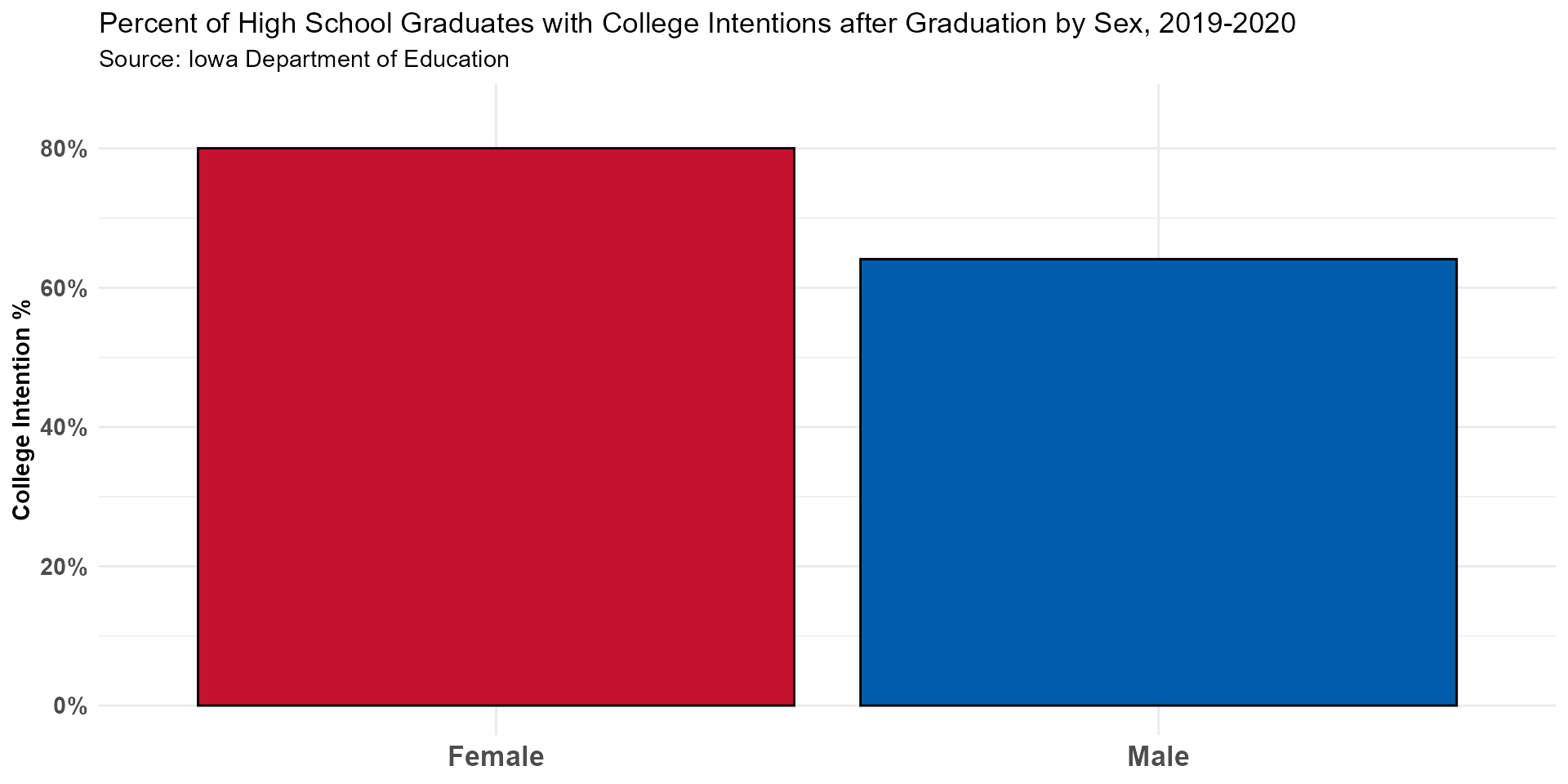

Download Graph: (SVG) (PNG)

Bottom-right graph: Percent of High School Graduates with College Intentions after Graduation by Race, 2019-2020

ds %>%
  filter(Group %in% c("White", "Black", "Hispanic", "Asian", "Pacific Islander", "Multi-Race"),
         Intention %in% c("Private 4-Year", "Public 4-Year", "Community College", "Private 2-Year")) %>%
  group_by(Group) %>%
  summarise(College = sum(Count)) %>%
  mutate(`Total Responses` = c(asian_responses, 
                               black_responses, 
                               hispanic_responses, 
                               multi_responses,
                               pi_responses,
                               white_responses),
         `College Rate` = College / `Total Responses`,
         `Non-college Responses` = `Total Responses` - College,
         `Non-college Rate` = 1 - `College Rate`) %>%
  ggplot(aes(x = reorder(Group, `College Rate`), y = `College Rate`)) + 
  geom_col(color = "black", fill = "#2A6EBB") +
  theme_minimal() +
  ylab("College Intention Percent") +
  labs(title = "Percent of High School Graduates with College Intentions after Graduation by Race, 2019-2020",
       subtitle = "Source: Iowa Department of Education") +
  scale_y_continuous(breaks = c(0, .20, .40, .60, .80),
                     labels = c("0%", "20%", "40%", "60%", "80%"),
                     limits = c(0,.85)) + 
  theme(legend.position = "none",
        axis.text = element_text(face = "bold", size = 11),
        axis.title = element_blank()) +
  geom_hline(yintercept = .720, color = "black", linetype = "dashed", size = 1) +
  annotate(geom = "text", x = 2.5, y = .755, label = "Overall Percent", fontface = "bold", size = 5)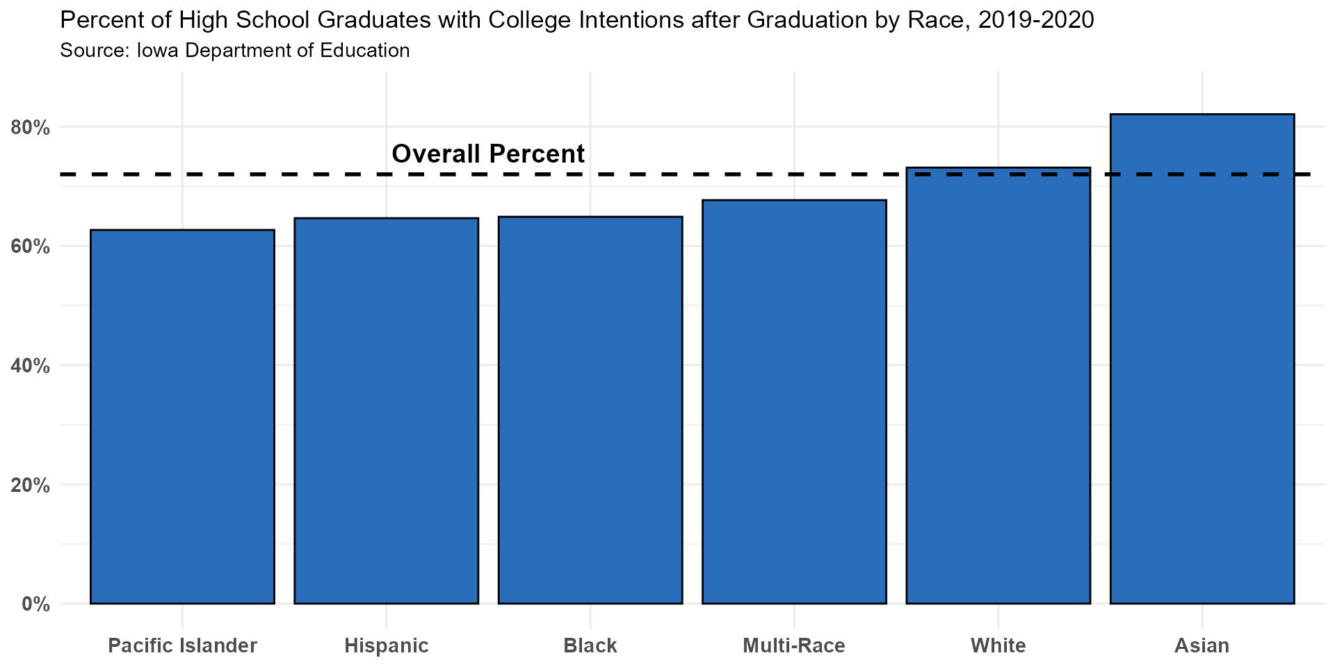

Download Graph: (SVG) (PNG)

Top-right map: Percent of High School Graduates with College Intentions after Graduation, 2018-2019

ggplot(schools, aes(fill = CR.Bins)) + 
  geom_sf(color = "white", aes(geometry = geometry)) +
  theme_map() +
  labs(title = "Percent of High School Graduates with College Intentions after Graduation, 2018-2019",
       subtitle = "Source: Iowa Department of Education") +
  scale_fill_brewer(palette = "Blues",
                    name = "College Intention %",
                    na.value = "#B3B3B3") +
  theme(legend.title = element_text(size = 8, face = "bold"),
        legend.text = element_text(size = 8),
        legend.position = "left")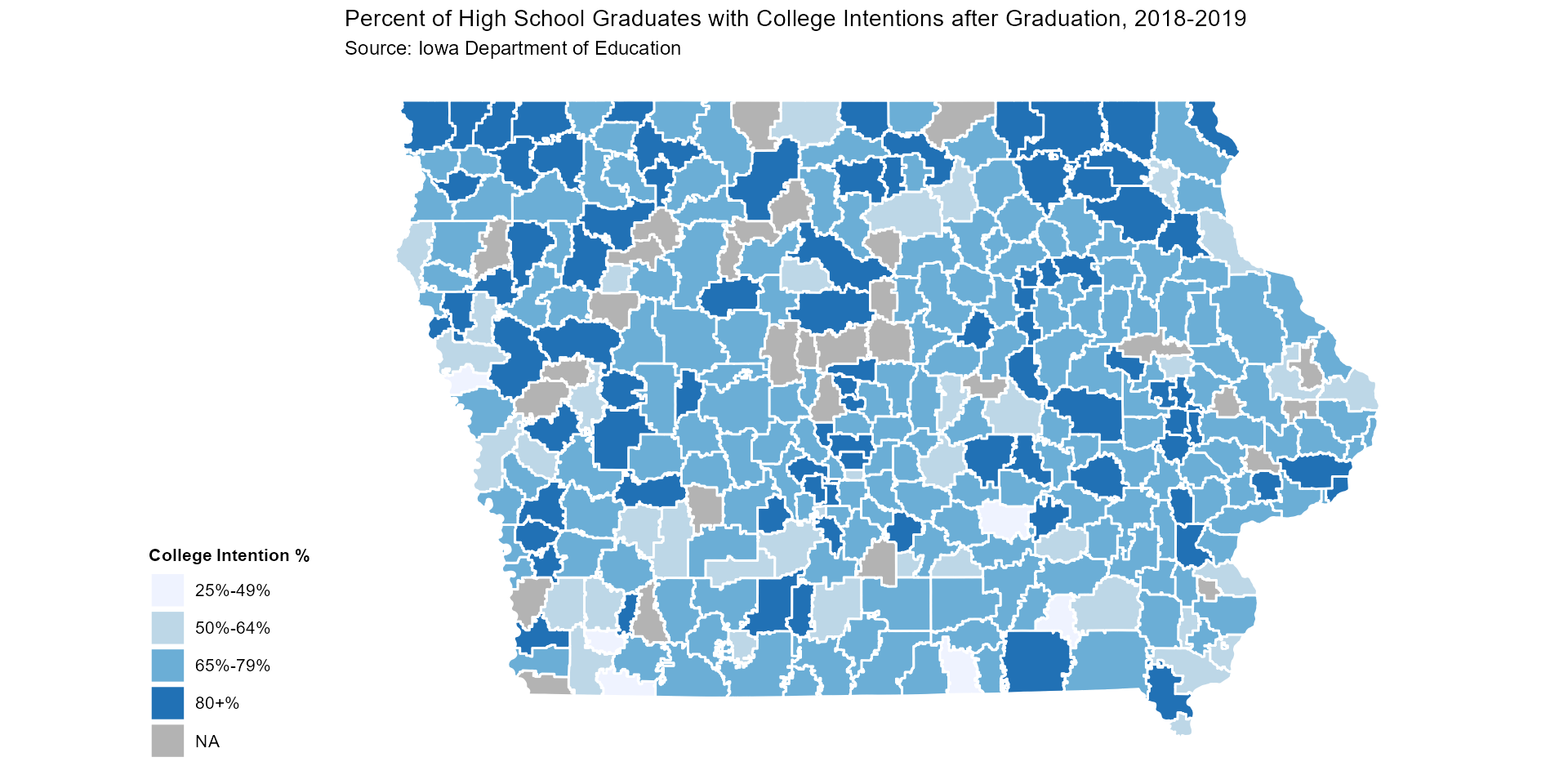

Download Graph: (SVG) (PNG)

Bottom-left graph: Percent of High School Graduates with College Intentions after Graduation, 2010-2019

college %>% 
  ggplot(aes(x = Year, y = Rate, color = Class)) +
  geom_line(size = 2) +
  scale_y_continuous(breaks = c(60, 65, 70, 75, 80, 85, 90, 95, 100),
                     labels = c("60%", "65%", "70%", "75%", "80%", "85%", "90%", "95%", "100%"),
                     limits = c(60 , 100)) +
  scale_x_continuous(breaks = c(2010, 2011, 2012, 2013, 2014, 2015, 2016, 2017, 2018, 2019),
                     labels = c(2010, 2011, 2012, 2013, 2014, 2015, 2016, 2017, 2018, 2019)) +
  labs(title = "Percent of High School Graduates with College Intentions after Graduation, 2010-2019",
       subtitle = "Source: Iowa Department of Education") +
  theme_minimal() +
  theme(axis.text = element_text(face = "bold", size = 11),
        axis.title = element_text(face = "bold", size = 11),
        axis.title.y = element_text(angle = 0, vjust = .5),
        legend.text = element_text(size = 11),
        legend.title = element_text(size = 11, face = "bold")) +
  scale_color_manual(name = "City Population", values = 
                       c("#CA0020", "#F4A582", "light grey", "#92C5DE", "#0571B0"))

Download Graph: (SVG) (PNG)