How Does Employment and Unemployment Compare Across Age, Sex, and Race/Ethnicity?
un_employmentByAgeSexRaceEthnicity.RmdThis is a supplementary vignette for the DHR Workforce Poster “How Does (Un)Employment Compare Across Age, Sex, and Race/Ethnicity?”
When analyzing unemployment rates, we rarely have up-to-date data that is stratified by Sex, Age, or Race/Ethnicity. Unemployment insurance claims can be used as a proxy for actual unemployment with the caveat that individuals who file for unemployment insurance are a subset of all unemployed individuals. Unemployment insurance claims data give a rough idea of which communities are experiencing the highest rates of unemployment.
Number of Continued Unemployment Insurance Claims by Sex
Download unemployment claims by Sex from Iowa Data Center. Note that the Iowa Data Center refers to Male/Female as “Genders” rather than “Sex,” so this is continued below.
library(tidyverse)

unemploymentClaimsByGender <- read_csv("../data_raw/Iowa_Unemployment_Insurance_Claimants_by_Gender__Monthly_.csv")
plt <- unemploymentClaimsByGender %>%
  select(-(`Not Available`)) %>%
  pivot_longer(cols = c("Male","Female"),
               names_to = "sex",
               values_to = "count") %>%
  mutate(Date = lubridate::mdy_hm(Month)) %>%
  mutate(Date = as.Date(as.character(Date))) %>%
  ggplot() +
  geom_line(aes(x = Date,y = count,colour = sex),size = 1.5) +
  theme_bw() +
  scale_colour_manual(values = c("#D81E3F","#2A6EBB")) +
  scale_y_continuous(labels = scales::comma,limits = c(NA,NA)) +
  scale_x_date(breaks = as.Date(paste0(c(seq(2000,2020,by = 5)),"-01-01",sep = "")),
               date_labels = "%Y") +
  labs(colour = "Sex"
  ) +
  theme(legend.position = "bottom",
        axis.title = element_blank(),
        axis.text = element_text(size = 19)
  ) +
  coord_cartesian(expand = FALSE)

plt +
  geom_rect(data = data.frame(xmin = as.Date("2019-01-01"),
                              xmax = as.Date("2021-05-31"),
                              ymin = 0,
                              ymax = unemploymentClaimsByGender %>%
                                select(-(`Not Available`)) %>%
                                pivot_longer(cols = c("Male","Female"),
                                             names_to = "sex",
                                             values_to = "count") %>%
                                pull(count) %>%
                                max()),
            aes(xmin = xmin,xmax = xmax,ymin = ymin,ymax = ymax),
            fill = "gray50",
            alpha = .5) +
  theme(legend.position = "bottom")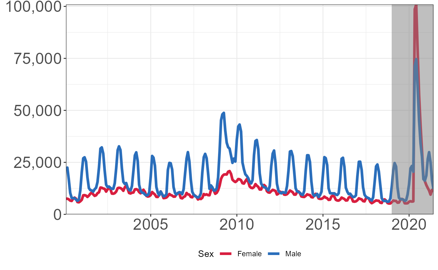
Show window from 1/1/19 to 5/31/2021.
plt +
  coord_cartesian(xlim = c(as.Date("2019-01-01"),as.Date("2021-05-31")),expand = FALSE) +
  scale_x_date(breaks = as.Date(paste0(c(seq(2019,2021,by = 1)),"-01-01",sep = "")),
               date_labels = "%Y") +
  theme(legend.position = "bottom")
#> Coordinate system already present. Adding new coordinate system, which will replace the existing one.
#> Scale for 'x' is already present. Adding another scale for 'x', which will
#> replace the existing scale.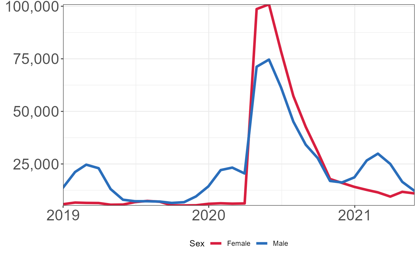
Same information as above, but show as percent of all claiments
unemploymentClaimsByGender_perc <- data.frame(unemploymentClaimsByGender) %>%
  mutate(percentMale = 100*Male/Total,
         percentFemale = 100*Female/Total,
         percentUnavailable = 100*Not.Available/Total)  %>%
  select(Month, contains("percent")) %>%
  pivot_longer(cols = contains("percent")) %>%
  mutate(date = lubridate::mdy_hm(Month))

plt <- unemploymentClaimsByGender_perc %>%
  filter(!(name %in% c("percentUnavailable"))) %>%
  mutate(date = as.Date(date)) %>%
  ggplot(aes(x = date, y = value, group = name, color = name)) +
  geom_line(size = 1.5) +
  # labs(title = "Sex Breakdown of Iowa Unemployment Insurance Claimants", x = "Date", y = "%", color = "") +
  theme_bw() +
  theme(legend.position = "bottom",
        axis.title = element_blank()) +
  scale_colour_manual(values = c("#D81E3F","#2A6EBB"))

plt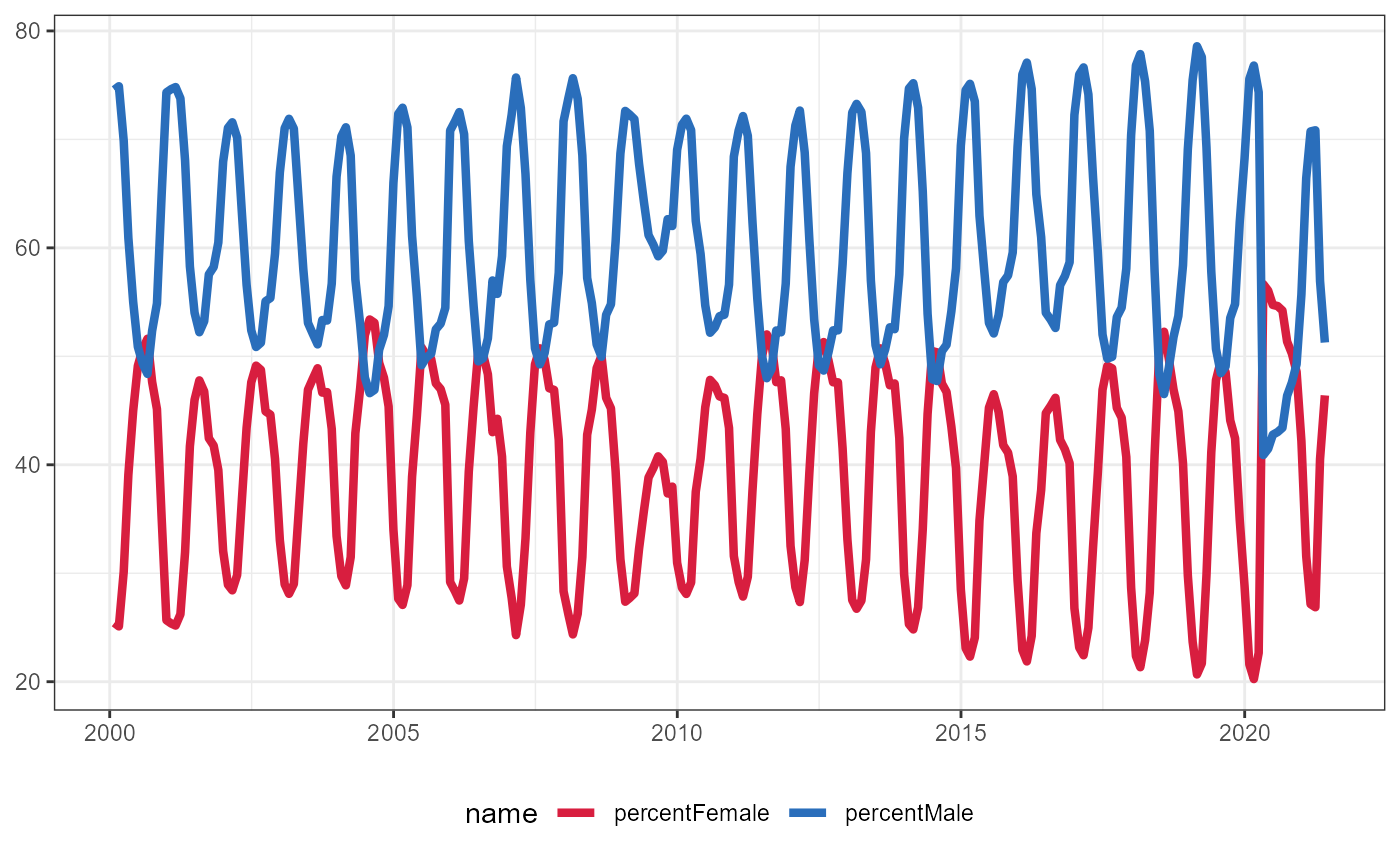
Show window from 1/1/19 to 5/31/21
plt +
  scale_x_date(limits = c(xmin = as.Date("2019-01-01"),
                          xmax = as.Date("2021-05-31")))
#> Warning: Removed 456 row(s) containing missing values (geom_path).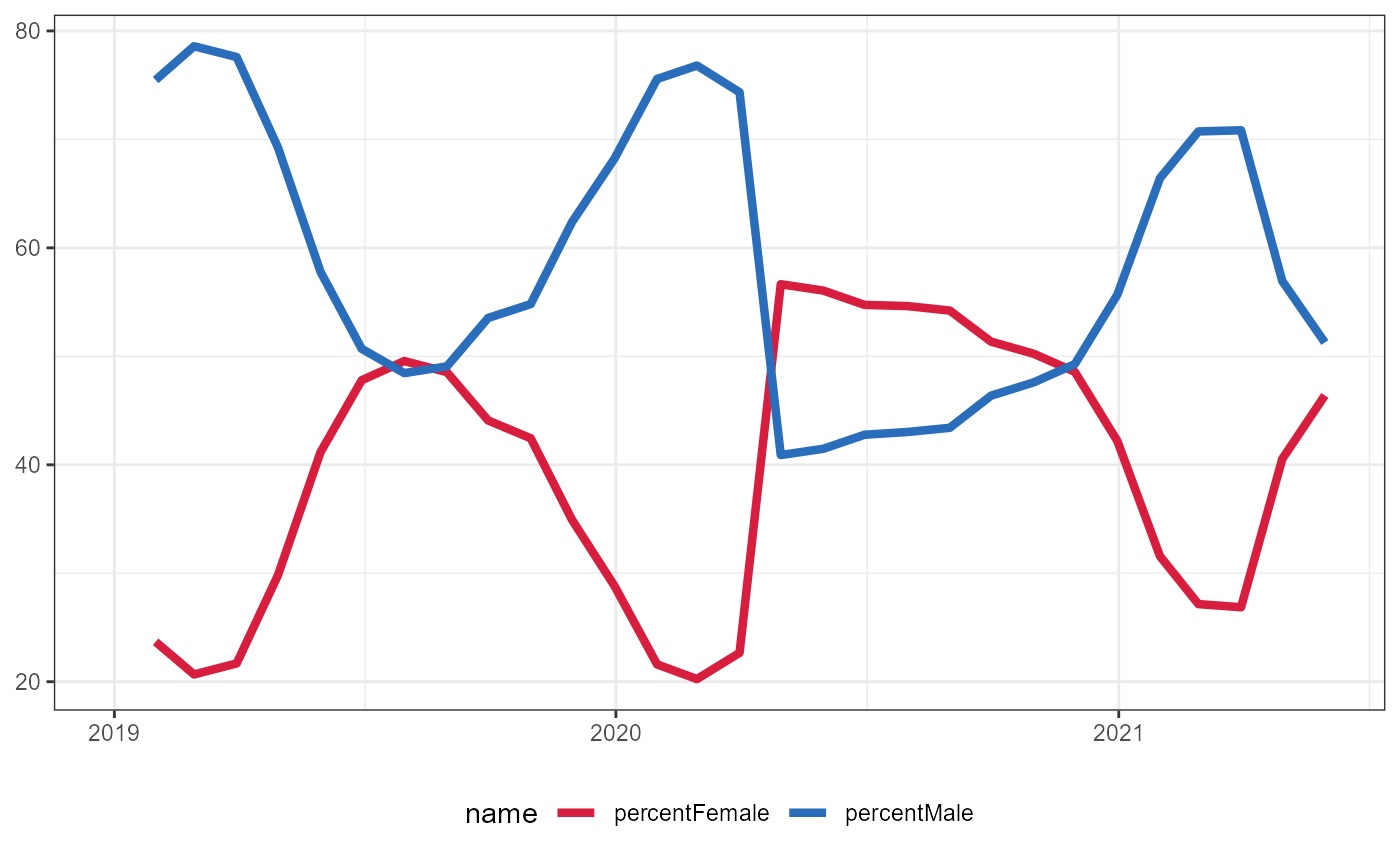
Same information as above, but show as a percent of all Males/Females
Note that we are using 2019 ACS 5-year survey estimate for the population of each Sex group. See Iowa Quick Facts.
plt <- unemploymentClaimsByGender %>%
  select(-(`Not Available`)) %>%
  pivot_longer(cols = c("Male","Female"),
               names_to = "sex",
               values_to = "count") %>%
  mutate(prop = ifelse(sex == "Male",count/1543045,
                       count/1564081),
         Date = lubridate::mdy_hm(Month)) %>%
  mutate(Date = as.Date(as.character(Date))) %>%
  ggplot() +
  geom_line(aes(x = Date,y = prop,colour = sex),size = 1.5) +
  theme_bw() +
  scale_colour_manual(values = c("#D81E3F","#2A6EBB")) +
  scale_y_continuous(labels = scales::percent,limits = c(0,NA)) +
  labs(colour = "Sex"
  ) +
  theme(legend.position = "bottom",
        axis.title = element_blank()
  ) +
  coord_cartesian(expand = FALSE)

plt +
  geom_rect(data = data.frame(xmin = as.Date("2019-01-01"),
                              xmax = as.Date("2021-05-31"),
                              ymin = 0,
                              ymax = unemploymentClaimsByGender %>%
                                select(-(`Not Available`)) %>%
                                pivot_longer(cols = c("Male","Female"),
                                             names_to = "sex",
                                             values_to = "count") %>%
                                mutate(prop = ifelse(sex == "Male",count/1543045,
                                                     count/1564081)) %>%
                                pull(prop) %>%
                                max()),
            aes(xmin = xmin,xmax = xmax,ymin = ymin,ymax = ymax),
            fill = "gray50",
            alpha = .5) +
  theme(legend.position = "bottom")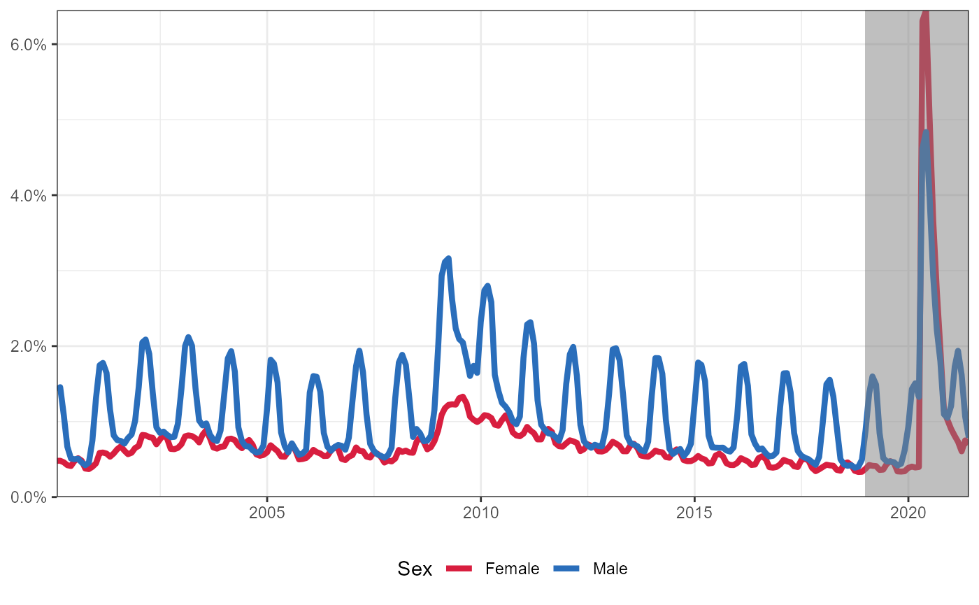
Show window from 1/1/19 to 5/31/2021.
plt +
  coord_cartesian(xlim = c(as.Date("2019-01-01"),as.Date("2021-05-31"))) +
  theme(legend.position = "bottom")
#> Coordinate system already present. Adding new coordinate system, which will replace the existing one.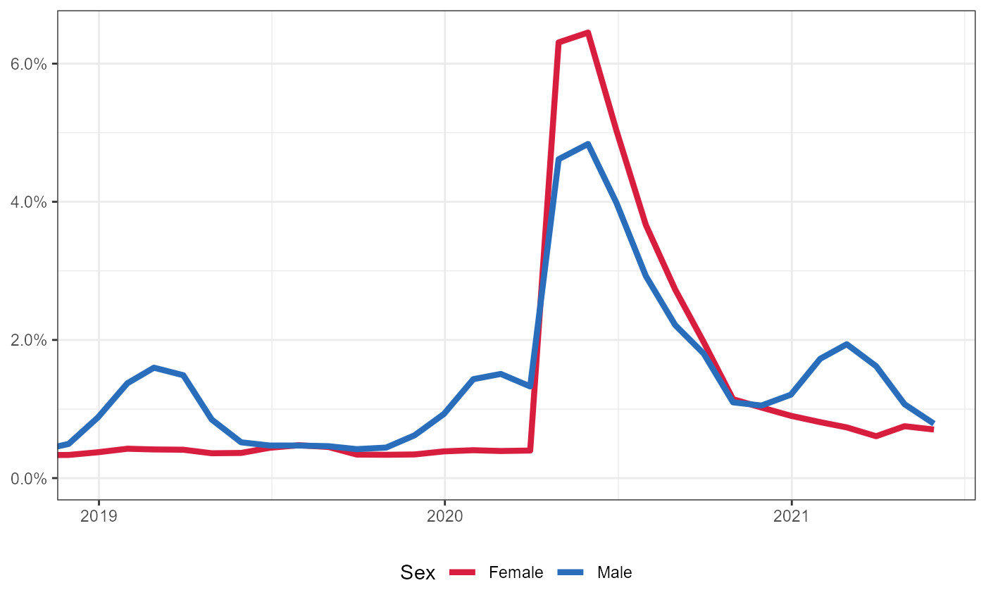
Number of Continued Unemployment Insurance Claims by Age Group
Download unemployment claims by age from Iowa Data Center.
unemploymentClaimsByAge <- read_csv("../data_raw/Iowa_Unemployment_Insurance_Claimants_by_Age__Monthly_.csv")
#>
#> -- Column specification --------------------------------------------------------
#> cols(
#>   Month = col_character(),
#>   Total = col_double(),
#>   `Under 22` = col_double(),
#>   `22-24` = col_double(),
#>   `25-34` = col_double(),
#>   `35-44` = col_double(),
#>   `45-54` = col_double(),
#>   `55-59` = col_double(),
#>   `60-64` = col_double(),
#>   `65 & over` = col_double(),
#>   INA = col_double()
#> )
plt <- unemploymentClaimsByAge %>%
  select(-INA) %>%
  pivot_longer(3:10,names_to = "ageGroup",values_to = "count") %>%
filter(!(ageGroup %in% c("Under 22","22-24","65 & over"))) %>%
  mutate(ageGroup2 = ifelse(ageGroup %in% c("25-34"),"25-34",
                            ifelse(ageGroup %in% c("55-59","60-64"),"55-64",
                                   ageGroup))) %>%
  group_by(ageGroup2,Month) %>%
  summarise(count = sum(count),
            .groups = "drop") %>%
  mutate(ageGroup2 = factor(ageGroup2,
                            levels = c("25-34","35-44","45-54","55-64")),
         Date = as.Date(as.character(lubridate::mdy_hm(Month)))) %>%
  ggplot() +
  geom_line(aes(x = Date,y = count,colour = ageGroup2),size = 1.5) +
  theme_bw() +
  theme(axis.title = element_blank(),
        legend.position = "bottom",
        axis.text = element_text(size = 19)) +
  scale_y_continuous(labels = scales::comma) +
  scale_colour_manual(values = c("gray25","gray50","#2A6EBB","#D81E3F")) +
  labs(colour = "Age Group") +
  guides(colour = guide_legend(nrow = 1))

plt +
  geom_rect(data = data.frame(xmin = as.Date("2019-01-01"),
                              xmax = as.Date("2021-05-31"),
                              ymin = 0,
                              ymax = 43027), #max number of claims made in a month
            aes(xmin = xmin,xmax = xmax,ymin = ymin,ymax = ymax),
            fill = "gray50",
            alpha = .5) +
  theme(legend.position = "bottom") +
  coord_cartesian(expand = FALSE)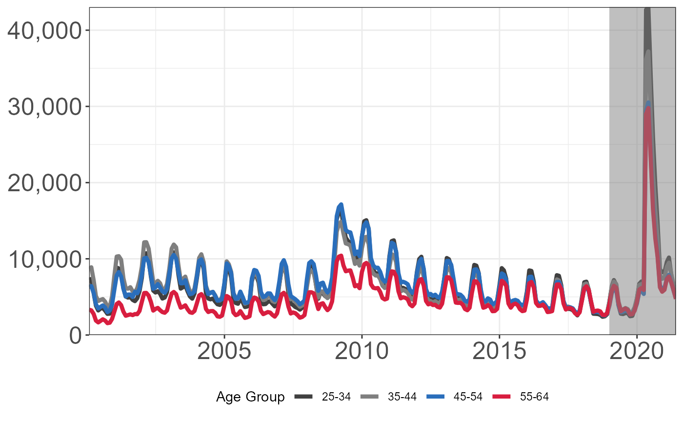
Show window from 1/1/19 to 5/31/21.
plt +
  coord_cartesian(xlim = c(as.Date("2019-01-01"),as.Date("2021-05-31")),
                  expand = FALSE) +
  theme(legend.position = "bottom")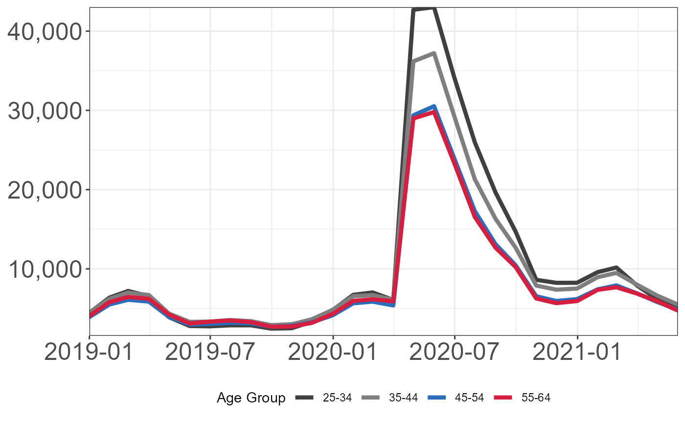
Same information as above, but show as percentage of total claims
plt <- unemploymentClaimsByAge %>%
  select(-INA) %>%
  pivot_longer(3:10,names_to = "ageGroup",values_to = "count") %>%
filter(!(ageGroup %in% c("Under 22","22-24","65 & over"))) %>%
  mutate(ageGroup2 = ifelse(ageGroup %in% c("25-34"),"25-34",
                            ifelse(ageGroup %in% c("55-59","60-64"),"55-64",
                                   ageGroup))) %>%
  group_by(ageGroup2,Month) %>%
  summarise(count = sum(count),
            .groups = "drop") %>%
  mutate(ageGroup2 = factor(ageGroup2,
                            levels = c("25-34","35-44","45-54","55-64")),
         Date = as.Date(as.character(lubridate::mdy_hm(Month)))) %>%
  group_by(Date) %>%
  mutate(total = sum(count),
         prop = count/total) %>%
  ggplot(aes(x = Date, y = prop, group = ageGroup2, color = ageGroup2)) +
  geom_line(size = 1.5) +
  theme_bw() +
  scale_y_continuous(labels = scales::percent) +
  theme(legend.position = "bottom",
        axis.title = element_blank()) +
  scale_colour_manual(values = c("gray25","gray50","#2A6EBB","#D81E3F")) +
  labs(colour = "Age Group")

plt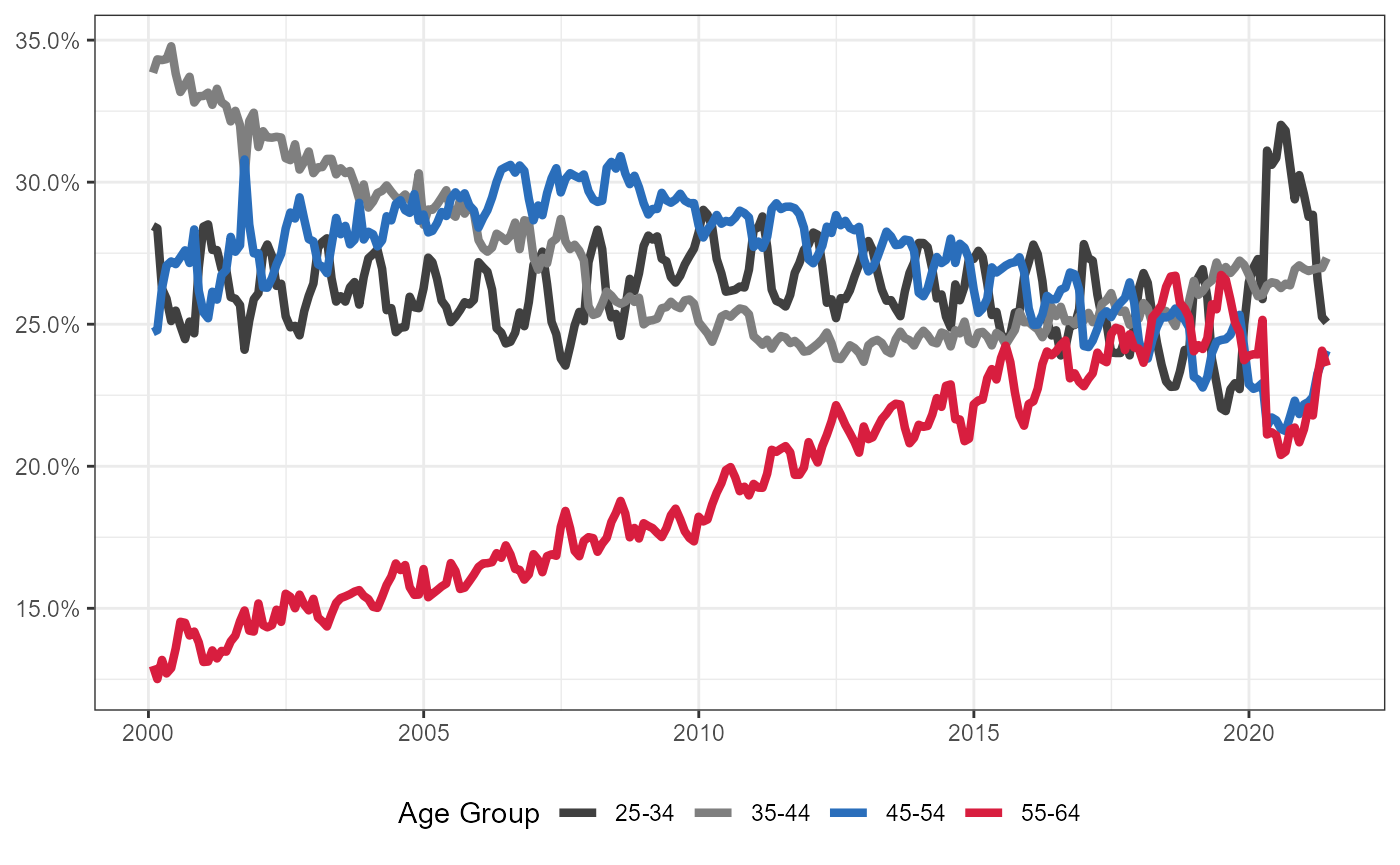
plt +
  coord_cartesian(xlim = c(as.Date("2019-01-01"),as.Date("2021-05-31")),
                  expand = FALSE) +
  theme(legend.position = "bottom")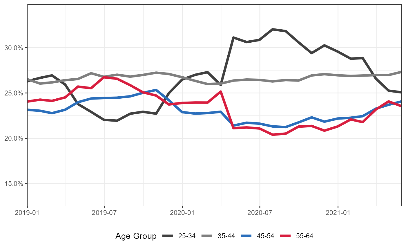
Same information as above, but show as a percentage of each age group population
Note that we are using 2019 ACS 5-year survey estimate for the population of each age group.
# Download from ACS, https://censusreporter.org/tables/B01001/
# ageTotals <- tidycensus::get_acs(geography = "state",table = "B01001",year = 2019,state = "IA",survey = "acs5")

# or load from the work repo
load("../data_raw/acs_ageGroup_estimates.RData")

# helper data set of ACS 5-year survey variables/codes
load("../data_clean/dataClean_acs5VariableLabels_acs5_2019.rda")

plt <- unemploymentClaimsByAge %>%
  select(-INA) %>%
  pivot_longer(3:10,names_to = "ageGroup",values_to = "count") %>%
  left_join(ageTotals %>%
              left_join(dataClean_acs5VariableLabels_acs5_2019 %>%
                          filter(year == 2019),
                        by = c("variable" = "name")) %>%
              filter(str_count(label,":!!") == 2) %>%
              tidyr::separate(col = label,into = c("label","sex","age"),sep = ":!!",remove = TRUE) %>%
              left_join(data.frame(age = c("Under 5 years","5 to 9 years","10 to 14 years","15 to 17 years","18 and 19 years","20 years","21 years",
                                           "22 to 24 years",
                                           "25 to 29 years","30 to 34 years",
                                           "35 to 39 years","40 to 44 years",
                                           "45 to 49 years","50 to 54 years",
                                           "55 to 59 years",
                                           "60 and 61 years","62 to 64 years",
                                           "65 and 66 years","67 to 69 years","70 to 74 years","75 to 79 years","80 to 84 years","85 years and over"
              ),
              ageGroup = c(rep("Under 22",times = 7),
                           rep("22-24",times = 1),
                           rep("25-34",times = 2),
                           rep("35-44",times = 2),
                           rep("45-54",times = 2),
                           rep("55-59",times = 1),
                           rep("60-64",times = 2),
                           rep("65 & over",times = 6)))) %>%
              group_by(ageGroup) %>%
              summarise(estimate = sum(estimate)),
            by = "ageGroup") %>%
  filter(!(ageGroup %in% c("Under 22","22-24","65 & over"))) %>%
  mutate(ageGroup2 = ifelse(ageGroup %in% c("25-34"),"25-34",
                            ifelse(ageGroup %in% c("55-59","60-64"),"55-64",
                                   ageGroup))) %>%
  group_by(ageGroup2,Month) %>%
  summarise(count = sum(count),
            estimate = sum(estimate),
            .groups = "drop") %>%
  mutate(ageGroup2 = factor(ageGroup2,
                            levels = c("25-34","35-44","45-54","55-64")),
         prop = count/estimate,
         Date = as.Date(as.character(lubridate::mdy_hm(Month)))) %>%
  ggplot() +
  geom_line(aes(x = Date,y = prop,colour = ageGroup2),size = 1.5) +
  theme_bw() +
  theme(axis.title = element_blank(),
        legend.position = "bottom") +
  scale_y_continuous(labels = scales::percent) +
  scale_colour_manual(values = c("gray25","gray50","#2A6EBB","#D81E3F")) +
  labs(colour = "Age Group") +
  guides(colour = guide_legend(nrow = 1))
#> Joining, by = "age"

plt +
  geom_rect(data = data.frame(xmin = as.Date("2019-01-01"),
                              xmax = as.Date("2021-05-31"),
                              ymin = 0,
                              ymax = 0.1089115),
            aes(xmin = xmin,xmax = xmax,ymin = ymin,ymax = ymax),
            fill = "gray50",
            alpha = .5) +
  coord_cartesian(expand = FALSE)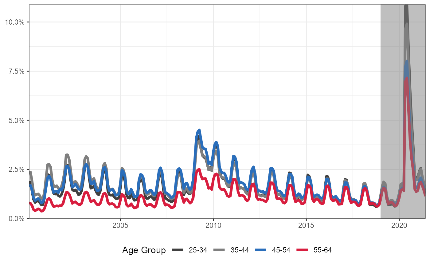
plt +
  coord_cartesian(xlim = c(as.Date("2019-01-01"),as.Date("2021-05-31")),
                  expand = FALSE)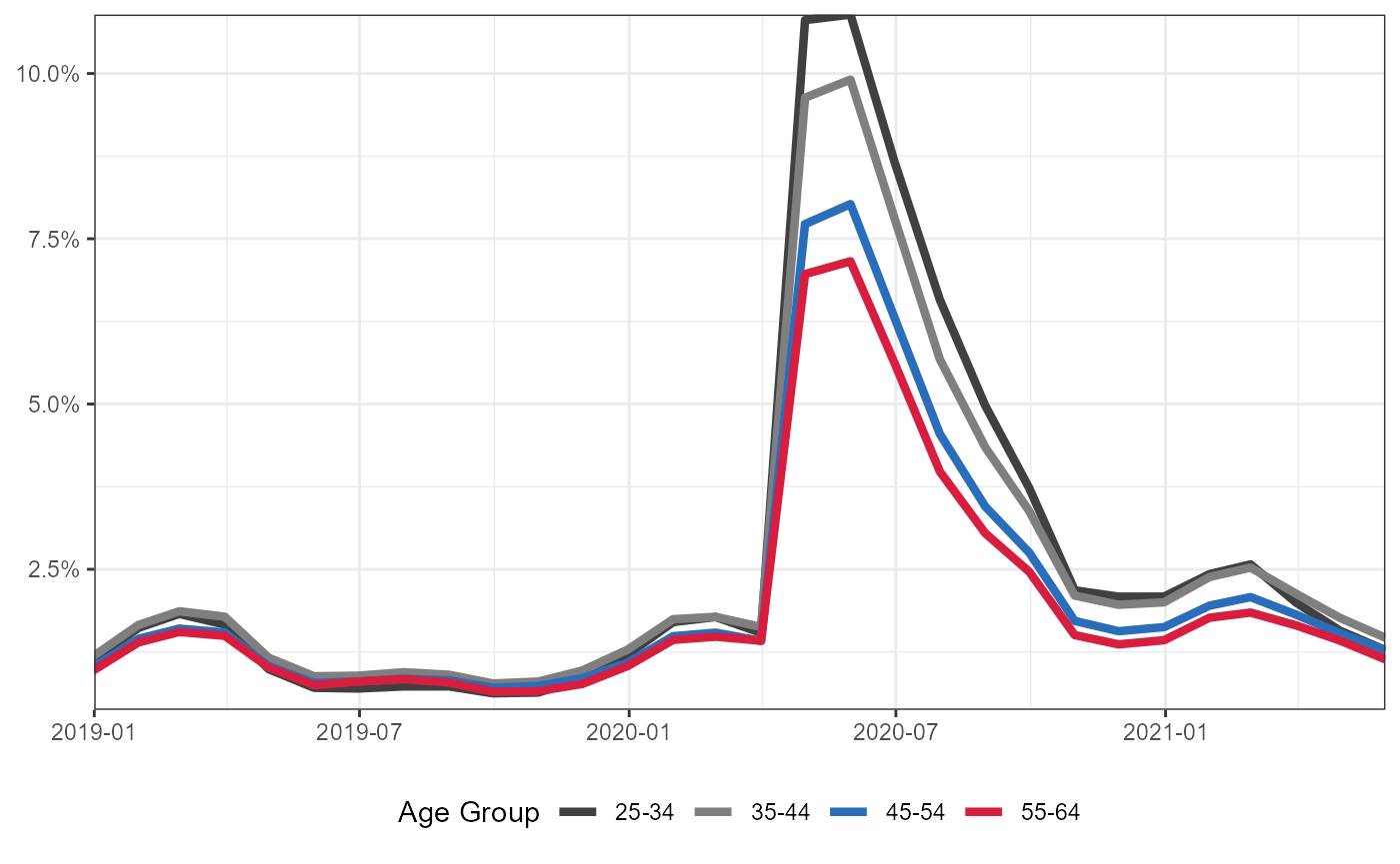
Number of Continued Unemployment Insurance Claims by Race/Ethnicity
Download unemployment claims by race/ethnicity from Iowa Data Center. Note that we only have data starting on unemployment insurance claims by race/ethnicity starting in 2019.
unemploymentClaimsByRace <- read_csv("../data_raw/Iowa_Unemployment_Insurance_Claimants_by_Race_and_Ethnicity.csv")
#>
#> -- Column specification --------------------------------------------------------
#> cols(
#>   MonthEndDate = col_character(),
#>   Total = col_double(),
#>   `American Indian or Alaska Native` = col_double(),
#>   Asian = col_double(),
#>   `Black or African American` = col_double(),
#>   `Native Hawaiian or Other Pacific Islander` = col_double(),
#>   White = col_double(),
#>   `Hispanic or Latino` = col_double(),
#>   `Information Not Available` = col_double()
#> )
unemploymentClaimsByRace %>%
  select(-c(`Native Hawaiian or Other Pacific Islander`,`Information Not Available`)) %>%
  pivot_longer(cols = 3:7,names_to = "label",values_to = "count") %>%
  mutate(label = tolower(label)) %>%
  mutate(Date = lubridate::mdy_hm(MonthEndDate),
         race = factor(ifelse(label == "american indian or alaska native","American Indian or\nAlaska Native",
                              ifelse(label == "black or african american","Black or\nAfrican American",
                                     ifelse(label == "hispanic or latino",
                                            "Hispanic or\nLatino",
                                            ifelse(label == "asian","Asian",
                                                   "White")))),
                       levels = c("American Indian or\nAlaska Native","Asian","Black or\nAfrican American",
                                  "White","Hispanic or\nLatino"))) %>%
  ggplot(aes(x = Date,y = count,colour = race)) +
  geom_line(size = 1.5) +
  theme_bw() +
  theme(legend.position = "bottom",
        axis.title = element_blank(),
        axis.text = element_text(size = 19)) +
  scale_colour_manual(values = c("gray25","gray50","gray75","#2A6EBB","#D81E3F")) +
  labs(colour = "Race/Ethnicity"
  ) +
  scale_y_log10(labels = scales::comma) +
  guides(colour = guide_legend(nrow = 2)) +
  coord_cartesian(expand = FALSE,ylim = c(100,200000))  +
  theme(legend.position = "bottom")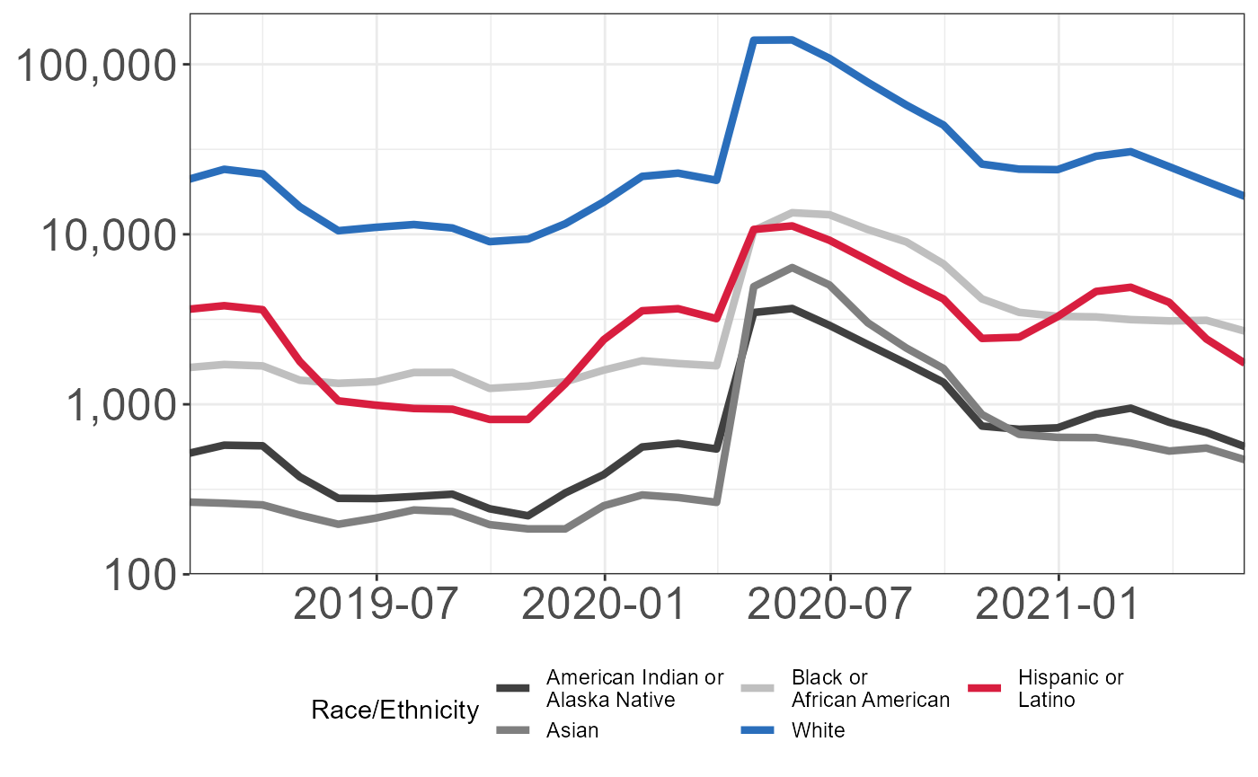
Same information as above, but show as percentage of total claims
Filter-out White claiments as they dominate the graph.
unemploymentClaimsByRace_perc <- data.frame(unemploymentClaimsByRace) %>%
  mutate(percentNativeAmerican = 100*American.Indian.or.Alaska.Native/Total,
         percentAsian = 100*Asian/Total,
         percentBlack = 100*Black.or.African.American/Total,
         percentPacificIslander = 100*Native.Hawaiian.or.Other.Pacific.Islander/Total,
         percentWhite = 100*White/Total, percentHispanic = 100*Hispanic.or.Latino/Total,
         percentUnavailable = 100*Information.Not.Available/Total)

unemploymentClaimsByRace_perc <- unemploymentClaimsByRace_perc %>%
  select(MonthEndDate, contains("percent")) %>%
  pivot_longer(cols = contains("percent")) %>%
  mutate(date = lubridate::mdy_hm(MonthEndDate))

unemploymentClaimsByRace_perc %>%
  filter(!(name %in% c("percentUnavailable","percentWhite"))) %>%
  mutate(value = value/100,
         date = as.Date(date),
         race = factor(ifelse(name == "percentNativeAmerican","American Indian or\nAlaska Native",
                              ifelse(name == "percentBlack","Black or\nAfrican American",
                                     ifelse(name == "percentHispanic",
                                            "Hispanic or\nLatino",
                                            ifelse(name == "percentAsian","Asian",
                                                   "White")))),
                       levels = c("American Indian or\nAlaska Native","Asian","Black or\nAfrican American",
                                  "White","Hispanic or\nLatino"))) %>%
  filter(race != "White") %>%
  ggplot(aes(x = date, y = value, group = race, color = race)) +
  geom_line() +
  theme_bw() +
  theme(text = element_text(family = "sans"),
        axis.title = element_blank(),
        axis.text = element_text(size = 19)) +
  scale_y_continuous(labels = scales::percent) +
  scale_colour_manual(values = c("gray25","gray75","#2A6EBB","#D81E3F")) +
  scale_x_date(breaks = as.Date(paste0(c(seq(2019,2021,by = 1)),"-01-01",sep = "")),
               date_labels = "%Y") +
  coord_cartesian(expand = FALSE)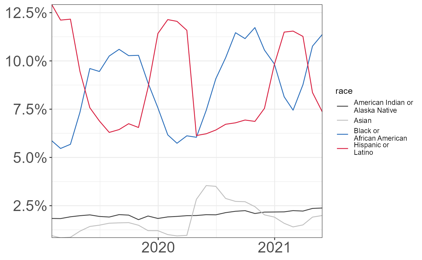
Same information as above, but show as a percentage of the race/ethnic group population
Note that we are using 2019 ACS 5-year survey estimate for the population of each race/ethnic group.
# download from ACS
# hispanicTotal <- tidycensus::get_acs(geography = "state",table = "B03002",year = 2019,state = "IA",survey = "acs5")

# or load from the work repo
load("../data_raw/acs_hispanic_estimates.RData")

# helper data set of ACS 5-year survey variables/codes
load("../data_clean/dataClean_acs5VariableLabels_acs5_2019.rda")

hispanicTotal %>%
  left_join(dataClean_acs5VariableLabels_acs5_2019 %>%
              filter(year == 2019),
            by = c("variable" = "name")) %>%
  filter(variable == "B03002_012")
#> # A tibble: 1 x 8
#>   GEOID NAME  variable  estimate   moe label              concept           year
#>   <chr> <chr> <chr>        <dbl> <dbl> <chr>              <chr>            <dbl>
#> 1 19    Iowa  B03002_0~   188311   135 Estimate!!Total:!~ HISPANIC OR LAT~  2019

# download from ACS
# raceTotal <- tidycensus::get_acs(geography = "state",table = "B02001",year = 2019,state = "IA",survey = "acs5")

#or load from the work repo
load("../data_raw/acs_race_estimates.RData")

totals <- bind_rows(raceTotal %>%
                      left_join(dataClean_acs5VariableLabels_acs5_2019 %>%
                                  filter(year == 2019),
                                by = c("variable" = "name")) %>%
                      filter(variable %in% c("B02001_002","B02001_003","B02001_004","B02001_005")) %>%
                      mutate(label = c("white","black or african american","american indian or alaska native","asian")) %>%
                      select(label,estimate),
                    hispanicTotal %>%
                      left_join(dataClean_acs5VariableLabels_acs5_2019 %>%
                                  filter(year == 2019),
                                by = c("variable" = "name")) %>%
                      filter(variable == "B03002_012") %>%
                      mutate(label = "hispanic or latino") %>%
                      select(label,estimate))
unemploymentClaimsByRace %>%
  select(-c(`Native Hawaiian or Other Pacific Islander`,`Information Not Available`)) %>%
  pivot_longer(cols = 3:7,names_to = "label",values_to = "count") %>%
  mutate(label = tolower(label)) %>%
  left_join(totals,
            by = "label") %>%
  mutate(prop = count/estimate,
         Date = lubridate::mdy_hm(MonthEndDate),
         race = factor(ifelse(label == "american indian or alaska native","American Indian or\nAlaska Native",
                              ifelse(label == "black or african american","Black or\nAfrican American",
                                     ifelse(label == "hispanic or latino",
                                            "Hispanic or\nLatino",
                                            ifelse(label == "asian","Asian",
                                                   "White")))),
                       levels = c("American Indian or\nAlaska Native","Asian","Black or\nAfrican American",
                                  "White","Hispanic or\nLatino"))) %>%
  ggplot(aes(x = Date,y = prop,colour = race)) +
  geom_line(size = 1.5) +
  theme_bw() +
  theme(legend.position = "bottom",
        axis.title = element_blank()) +
  scale_colour_manual(values = c("gray25","gray50","gray75","#2A6EBB","#D81E3F")) +
  labs(colour = "Race/Ethnicity"
  ) +
  scale_y_continuous(labels = scales::percent) +
  guides(colour = guide_legend(nrow = 3)) +
  coord_cartesian(expand = FALSE)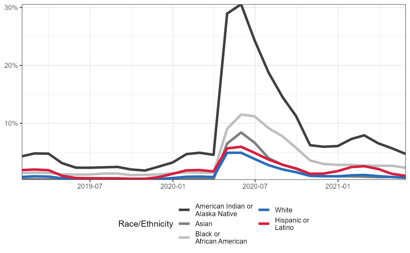
Occupation by Race and Ethnicity
Note that we are using 2019 ACS 1-year survey estimates.
# download data from ACS
# occupBySexRace <- map_dfr(c("A","B","C","D","E","F","H","I"),
#                           ~ {
#
#                             tidycensus::get_acs(geography = "state",state = "IA",table = paste0("B24010",.),survey = "acs1")
#
#                           })

# or load from the work repo
load("../data_raw/occupation_by_sexRace.RData")

# helper function of ACS 1-year survey variables/codes
load("../data_clean/dataClean_acs1VariableLabels_acs5_2019.rda")

occupByRace_summ <- occupBySexRace %>%
  left_join(dataClean_acs1VariableLabels_acs5_2019 %>%
              filter(year == 2019),
            by = c("variable" = "name")) %>%
  mutate(race = concept %>%
           map_chr(~ tolower(str_remove(str_split(string = .,pattern = "\\(")[[1]][2],
                                        pattern = " ALONE\\)")[[1]][1])))  %>%
  filter(!is.na(estimate)) %>%
  filter(str_count(label,":!!") == 4) %>%
  separate(label,into = c("lab","sex","occupHier1","occupHier2","occupHier3"),sep = ":!!") %>%
  group_by(race) %>%
  mutate(raceTotal = sum(estimate,na.rm = TRUE),
         raceTotalMOE = tidycensus::moe_sum(moe,estimate,na.rm = TRUE)) %>%
  group_by(occupHier3,race) %>%
  summarise(estimate = sum(estimate,na.rm = TRUE),
            moe = tidycensus::moe_sum(moe,estimate,na.rm = TRUE),
            raceTotal = unique(raceTotal),
            raceTotalMOE = unique(raceTotalMOE)
  ) %>%
  mutate(raceProp = estimate/raceTotal,
         racePropMOE = tidycensus::moe_prop(num = estimate,denom = raceTotal,moe_num = moe,moe_denom = raceTotalMOE)
  ) %>%
  mutate(raceFlag = racePropMOE > .5*raceProp
  ) %>%
  mutate(race = str_remove(race,"\\)")) %>%
  ungroup()
#> `summarise()` has grouped output by 'occupHier3'. You can override using the `.groups` argument.

popularOccupRace <- occupByRace_summ %>%
  group_by(race) %>%
  arrange(desc(raceProp)) %>%
  slice(1:3) %>%
  pull(occupHier3) %>%
  unique()

occupByRace_summ %>%
  filter(occupHier3 %in% popularOccupRace) %>%
  select(occupHier3,race,raceProp) %>%
  bind_rows(occupByRace_summ %>%
              filter(occupHier3 %in% popularOccupRace) %>%
              group_by(race) %>%
              mutate(occupHier3 = "Other",
                     raceProp = 1 - sum(raceProp)) %>%
              select(occupHier3,race,raceProp) %>%
              distinct()) %>%
  mutate(occupHier3 = str_remove(str_remove(occupHier3," occupations")," alone"),
         race = str_remove(race," alone")) %>%
  filter(race != "white") %>%
  group_by(race) %>%
  mutate(ymax = cumsum(raceProp)) %>%
  mutate(ymin = c(0,ymax[1:(length(ymax) - 1)])) %>%
  group_by(occupHier3,race) %>%
  mutate(yLabel = 1 - mean(c(ymin,ymax)),
        pltLabel = paste0(round(raceProp,2)*100,"%")) %>%
  mutate(race = factor(ifelse(race == "white, not hispanic or latino","White\nOnly",
                       ifelse(race == "hispanic or latino","Hispanic or\nLatino",
                              ifelse(race == "black or african american","African\nAmerican",
                                     "Asian"))),
                       levels = c("Asian","African\nAmerican","Hispanic or\nLatino","White\nOnly")),
         occupHier3 = ifelse(occupHier3 == "Health diagnosing and treating practitioners and other technical","Health diagnosing and treating\npractitioners and other technical",
                             ifelse(occupHier3 == "Business and financial operations","Business and financial\noperations",
                                    ifelse(occupHier3 == "Educational instruction, and library","Educational instruction, and library",
                                           occupHier3)))) %>%
  ungroup()  %>%
  ggplot(aes()) +
  geom_bar(aes(x = race,y = raceProp,fill = occupHier3),
           stat = "identity",colour = "black") +
  geom_text(aes(x = race,y = yLabel,label = pltLabel)) +
  coord_flip(expand = FALSE) +
  # coord_cartesian(expand = FALSE) +
  theme_bw() +
  theme(legend.position = "bottom",
        axis.title = element_blank()) +
  scale_y_continuous(labels = scales::percent) +
  colorspace::scale_fill_discrete_qualitative(palette = "Set 2") +
  guides(fill = guide_legend(ncol = 3,title = NULL,reverse = TRUE,label.position = "left",label.theme = element_text(size = 7,margin = margin(1.5,0,1.5,0))))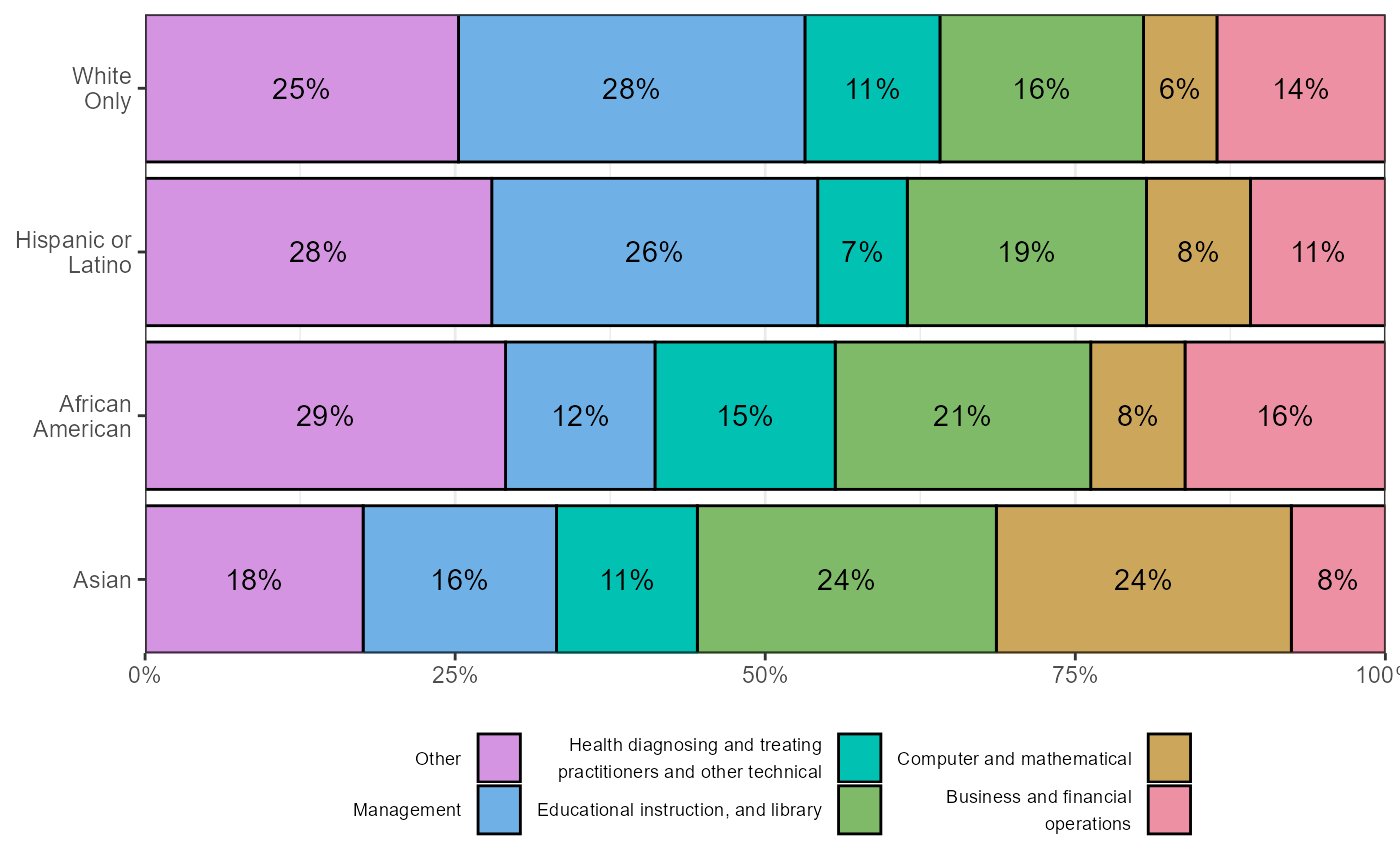
Occupation by Sex
Note that we are using 2019 ACS 1-year survey estimates.
occupBySex_summ <- occupBySexRace %>%
  left_join(dataClean_acs1VariableLabels_acs5_2019 %>%
              filter(year == 2019),
            by = c("variable" = "name")) %>%
  mutate(race = concept %>%
           map_chr(~ tolower(str_remove(str_split(string = .,pattern = "\\(")[[1]][2],
                                        pattern = " ALONE\\)")[[1]][1])))  %>%
  filter(!is.na(estimate)) %>%
  filter(str_count(label,":!!") == 4) %>%
  separate(label,into = c("lab","sex","occupHier1","occupHier2","occupHier3"),sep = ":!!") %>%
  group_by(sex) %>%
  mutate(sexTotal = sum(estimate),
         sexTotalMOE = tidycensus::moe_sum(moe,estimate)) %>%
  group_by(occupHier3,sex) %>%
  summarise(estimate = sum(estimate,na.rm = TRUE),
            moe = tidycensus::moe_sum(moe,estimate,na.rm = TRUE),
            sexTotal = unique(sexTotal),
            sexTotalMOE = unique(sexTotalMOE)
  ) %>%
  mutate(
         sexProp = estimate/sexTotal,
         sexPropMOE = tidycensus::moe_prop(num = estimate,denom = sexTotal,moe_num = moe,moe_denom = sexTotalMOE)
  ) %>%
  mutate(
         sexFlag = sexPropMOE > .5*sexProp
  ) %>%
  ungroup()
#> `summarise()` has grouped output by 'occupHier3'. You can override using the `.groups` argument.

popularOccupSex <- occupBySex_summ %>%
  group_by(sex) %>%
  arrange(desc(sexProp)) %>%
  slice(1:3) %>%
  pull(occupHier3) %>%
  unique()

occupBySex_summ %>%
  filter(occupHier3 %in% popularOccupSex) %>%
  select(occupHier3,sex,sexProp) %>%
  bind_rows(occupBySex_summ %>%
              filter(occupHier3 %in% popularOccupSex) %>%
              group_by(sex) %>%
              mutate(occupHier3 = "Other",
                     sexProp = 1 - sum(sexProp)) %>%
              select(occupHier3,sex,sexProp) %>%
              distinct()) %>%
  mutate(occupHier3 = str_remove(str_remove(occupHier3," occupations")," alone"),
         sex = str_remove(sex," alone")) %>%
  # filter(sex != "white") %>%
  group_by(sex) %>%
  mutate(ymax = cumsum(sexProp)) %>%
  mutate(ymin = c(0,ymax[1:(length(ymax) - 1)])) %>%
  group_by(occupHier3,sex) %>%
  mutate(yLabel = 1 - mean(c(ymin,ymax)),
        pltLabel = paste0(round(sexProp,2)*100,"%")) %>%
  mutate(occupHier3 = ifelse(occupHier3 == "Health diagnosing and treating practitioners and other technical","Health diagnosing and treating\npractitioners and other technical",
                             ifelse(occupHier3 == "Business and financial operations","Business and financial\noperations",
                                    ifelse(occupHier3 == "Educational instruction, and library","Educational instruction,\nand library",
                                           occupHier3)))) %>%
  ungroup()  %>%
  ggplot(aes()) +
  geom_bar(aes(x = sex,y = sexProp,fill = occupHier3),
           stat = "identity",colour = "black") +
  geom_text(aes(x = sex,y = yLabel,label = pltLabel)) +
  coord_flip(expand = FALSE) +
  # coord_cartesian(expand = FALSE) +
  theme_bw() +
  theme(legend.position = "bottom",
        axis.title = element_blank()) +
  scale_y_continuous(labels = scales::percent) +
  colorspace::scale_fill_discrete_qualitative(palette = "Set 2") +
  guides(fill = guide_legend(ncol = 3,title = NULL,reverse = TRUE,label.position = "right"))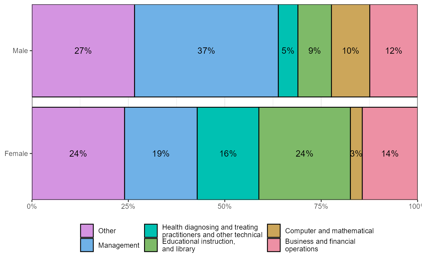
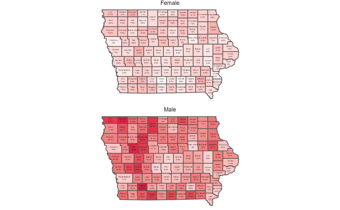
Rates of Self-Employment by Sex and County, 2019
# download from ACS
# sex_by_employment_type <- get_acs(geography = "county",
#                                   state = "IA",
#                                   variables = c(total = "B24080_001", male_total = "B24080_002", female_total = "B24080_012",
#                                                 male_selfemployed_incorporated = "B24080_005", male_selfemployed_unincorporated = "B24080_010",
#                                                 female_selfemployed_incorporated = "B24080_015", female_selfemployed_unincorporated = "B24080_020"))

# or load from the work repo
load("../data_raw/sex_by_employment_type.RData")

# helper data set containing county .shp information
load("../data_clean/dataClean_countyGeometry_acs5_2019.rda")


sex_by_employment_type <- sex_by_employment_type %>%
  select(-moe) %>%
  pivot_wider(names_from = variable, values_from = estimate) %>%
  mutate(male_selfemployed_total = male_selfemployed_incorporated + male_selfemployed_unincorporated,
         female_selfemployed_total = female_selfemployed_incorporated + female_selfemployed_unincorporated,
         workforce_percent_selfemployed = 100*(male_selfemployed_total + female_selfemployed_total)/total,
         percent_males_selfemployed = 100*male_selfemployed_total/male_total,
         percent_females_selfemployed = 100*female_selfemployed_total/female_total,
         diff_percent = percent_males_selfemployed - percent_females_selfemployed) %>%
  left_join(dataClean_countyGeometry_acs5_2019, by = "NAME")
sex_by_employment_type %>%
  select(NAME,geometry,percent_males_selfemployed,percent_females_selfemployed) %>%
  mutate(county = str_remove(NAME," County, Iowa"),
         Male = percent_males_selfemployed/100,
         Female = percent_females_selfemployed/100) %>%
  pivot_longer(cols = c(Male,Female),
               names_to = "sex") %>%
  mutate(pltLabel = paste0(county,"\n",round(value,3)*100,"%")) %>%
  ggplot(aes(geometry = geometry)) +
  geom_sf(aes(fill = value)) +
  geom_sf_text(aes(label = pltLabel),fun.geometry = sf::st_centroid,size = 1) +
  scale_fill_gradient(low = "white",high = "#D81E3F") +
  facet_wrap(~ sex,ncol = 1) +
  theme_void() +
  theme(
    legend.position = "none") +
  coord_sf(crs = sf::st_crs("NAD83"))
#> Warning in st_centroid.sfc(data$geometry): st_centroid does not give correct
#> centroids for longitude/latitude data

#> Warning in st_centroid.sfc(data$geometry): st_centroid does not give correct
#> centroids for longitude/latitude data