What are the Employment Characteristics of Iowans with Disabilities?
disabilityEmploymentCharacteristics.RmdThis is a supplementary vignette for the DHR Workforce Poster “What are the Employment Characteristics of Iowans with Disabilities?”
Individuals with disabilities participate in the labor force at lower rates than individuals without disabilities. By identifying top industries worked by individuals with disabilities and other economic opportunities, we can engage in informed intervention to help them participate in the labor force more fully.
Disability count bubble chart
See, e.g., the ACS Table #B18120 for estimates on the number of Iowans with disabilities.
library(tidyverse)

data.frame(x = c(1,1.4,1.96,2.46,2.8,3.3),
           y = rep(c(2,1),times = 3),
           lab = c("Ambulatory","Cognitive","Hearing","Indep. Living","Self-Care","Vision"),
           val = c(71577,85482,34670,61975,28589,25446),
           valStr = c("71,577","85,482","34,670","61,975","28,589","25,446")) %>%
  mutate(pltLabel = paste0(lab,"\n",valStr)) %>%
  ggplot(aes(x = x,y = y)) +
  geom_point(aes(size = val),colour = "black",shape = 21,fill = "#ddeaf9") +
  geom_text(aes(label = pltLabel),size = 3.5) +
  theme_void() +
  theme(legend.position = "none"
        # ,panel.background = element_rect(fill = "#eeeeeeff")
        ) +
  coord_fixed(xlim = c(0,5),
              ylim = c(0,3)) +
  scale_size(range = c(25,45))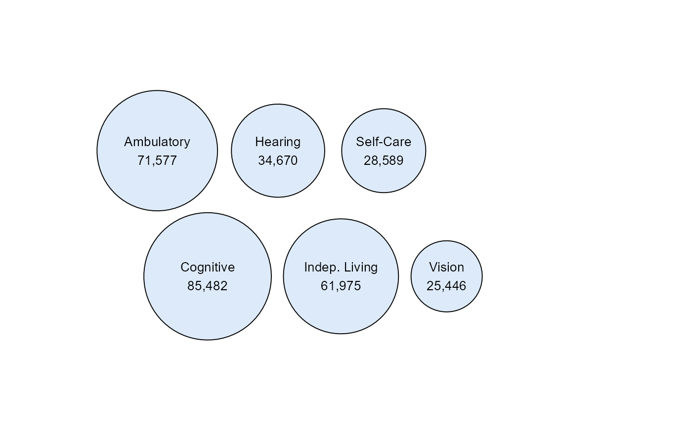
Median Earnings in the Last 12 Months by Disability Status & Sex Among Individuals 16+ Years of Age with Earnings
ACS 1-year estimates for 2010-2019 table B18140: Median Earnings by Disability Status by Sex for the Civilian Noninstitutionalized Population With Earnings are being loaded
library(tidyverse)

# can download data from ACS -- also available in the work repo
load("../data_raw/dataRaw_tenYearDisabilityIncome_acs1_2010_2011_2012_2013_2014_2015_2016_2017_2018_2019.rda")

# helper data set of ACS 1-year survey variable codes/names
load("../data_clean/dataClean_acs1VariableLabels_acs5_2019.rda")
variableNames_acs1 <- dataClean_acs1VariableLabels_acs5_2019

clean_disabilityIncome <- dataRaw_tenYearDisabilityIncome_acs1_2010_2011_2012_2013_2014_2015_2016_2017_2018_2019 %>%
  filter(variable %in% c("B18140_003","B18140_004","B18140_006","B18140_007"))%>%
  left_join(variableNames_acs1, by = c("variable" = "name", "year"="year"))%>%
  mutate(type=if_else(variable=="B18140_003", "Disabled Male",
                      if_else(variable=="B18140_004", "Disabled Female",
                              if_else(variable=="B18140_006", "Non-Disabled Male", "Non-Disabled Female"))))
clean_disabilityIncome %>%
  filter(year == 2019) %>%
  tidyr::separate(col = type,into = c("status","sex"),sep = " ",remove = FALSE) %>%
  ggplot(aes(x = sex, y = estimate, fill=sex)) +
  geom_bar(stat = "identity",colour = "black") +
  scale_colour_manual(values = c("#D81E3F","#2A6EBB","#D81E3F","#2A6EBB"),
                      aesthetics = c("fill","colour")) +
  theme_bw() +
  scale_y_continuous(labels=scales::dollar_format(),limits = c(0,50000)) +
  theme(legend.position = "none") +
  theme(text = element_text(family = "sans"),
        panel.background = element_rect(fill="white"),
        plot.background = element_rect(fill="white"),
        strip.background = element_rect(fill = NA),
        axis.title = element_blank(),
        panel.grid.major.x = element_blank()) +
  coord_cartesian(expand = FALSE,ylim = c(0,47500)) +
  facet_grid(cols = vars(status)) +
  geom_text(data = data.frame(status = rep(c("Disabled","Non-Disabled"),each = 2),
                               sex = rep(c("Female","Male"),times = 2),
                               y = c(15991,25674,30628,44037),
                               pltLabel = paste0("$",c("15,991","25,674","30,628","44,037"))),
             aes(x = sex,y = y,fill = sex,label = pltLabel),
            nudge_y = 2000)
#> Warning: Ignoring unknown aesthetics: fill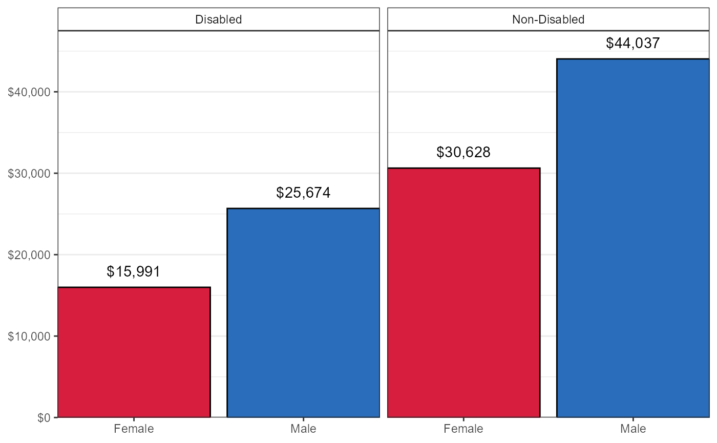
Time series of the same data as above from 2010-2019
clean_disabilityIncome %>%
  tidyr::separate(col = type,into = c("status","sex"),sep = " ",remove = FALSE) %>%
  ggplot(aes(year, estimate, color=sex)) +
  geom_line(size = 2) +
  scale_colour_manual(values = c("#D81E3F","#2A6EBB","#D81E3F","#2A6EBB"),
                      aesthetics = c("fill","colour")) +
  theme_bw() +
  scale_y_continuous(labels=scales::dollar_format(),limits = c(0,50000)) +
  scale_x_continuous(breaks = 2010:2019,labels = paste0("'",10:19),limits = c(2009.7,2019.3)) +
  theme(legend.position = "top")+
  theme(text = element_text(family = "sans"),
        panel.background = element_rect(fill="white"),
        plot.background = element_rect(fill="white"),
        strip.background = element_rect(fill = NA)) +
  coord_cartesian(expand = FALSE,ylim = c(0,47000),xlim = c(NA,2019.5)) +
  facet_grid(cols = vars(status)) +
  geom_point(data = data.frame(status = rep(c("Disabled","Non-Disabled"),each = 2),
                               x = 2019,
                               sex = rep(c("Female","Male"),times = 2),
                               y = c(15991,25674,30628,44037)),
             aes(x = x,y = y,colour = sex),size = 4) +
  geom_text(data = data.frame(status = rep(c("Disabled","Non-Disabled"),each = 2),
                               x = 2019,
                               sex = rep(c("Female","Male"),times = 2),
                               y = c(14500,23700,33000,46000),
                               pltLabel = paste0("$",c("15,991","25,674","30,628","44,037"))),
             aes(x = x,y = y,colour = sex,label = pltLabel),nudge_x = -.5)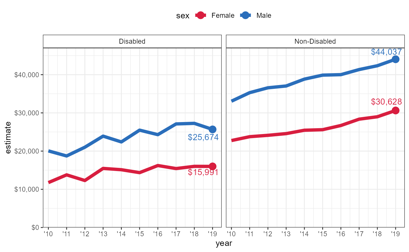
Percent of Individuals in the Labor Force Among Iowa’s Civilian, Non-Institutionalized Population Ages 18-64 by Disability Type, 2019
# download from ACS
# laborByDisability <- tidycensus::get_acs(geography = "state",year = 2019,table = "B18120",state = "IA",survey = "acs1")

# or load from the work repo
load("../data_raw/laborParticipationByDisability.RData")

load("../data_clean/dataClean_acs1VariableLabels_acs5_2019.rda")

# Iowa total proportion out of labor force (among 18-64 year-olds)
laborByDisability %>%
  left_join(dataClean_acs1VariableLabels_acs5_2019 %>%
              filter(year == 2019),
            by = c("variable" = "name")) %>%
  filter(str_detect(label,"No disability")) %>%
  mutate(total = sum(estimate))
#> # A tibble: 3 x 9
#>   GEOID NAME  variable  estimate   moe label          concept        year  total
#>   <chr> <chr> <chr>        <dbl> <dbl> <chr>          <chr>         <dbl>  <dbl>
#> 1 19    Iowa  B18120_0~  1405451 11025 Estimate!!Tot~ EMPLOYMENT S~  2019 1.68e6
#> 2 19    Iowa  B18120_0~    45969  3840 Estimate!!Tot~ EMPLOYMENT S~  2019 1.68e6
#> 3 19    Iowa  B18120_0~   232161  6471 Estimate!!Tot~ EMPLOYMENT S~  2019 1.68e6

laborPropByDisability <- laborByDisability %>%
  left_join(dataClean_acs1VariableLabels_acs5_2019 %>%
              filter(year == 2019),
            by = c("variable" = "name")) %>%
  filter(str_count(label,":!!") >= 3 & str_detect(label,"With a disability:!!")) %>%
  mutate(label = str_remove(label,"Employed:!!")) %>%
  mutate(label = str_remove(label,"Unemployed:!!")) %>%
  separate(col = label,into = c("lab","inLabor","withDisab","disabType"),sep = ":!!") %>%
  select(-c(lab,withDisab)) %>%
  mutate(disabType = str_remove(str_remove(str_remove(disabType," difficulty$"),"^With a "),"^With an ")) %>%
  group_by(disabType) %>%
  mutate(total = sum(estimate)) %>%
  filter(inLabor == "Not in labor force") %>%
  mutate(prop = estimate/total)

bind_rows(laborPropByDisability %>%
            select(disabType,prop),
          data.frame(disabType = "No Disability",
           prop = 232161/1683581)) %>%
  # look at percent IN labor force, not out
  mutate(prop = 1 - prop) %>%
  mutate(disabType = factor(disabType,
                            # levels = c("No Disability","ambulatory","cognitive","hearing","independent living","self-care","vision"),
                            levels = c("cognitive","ambulatory","independent living","hearing","self-care","vision","No Disability"),
                            labels = c("Cognitive","Ambulatory","Independent Living","Hearing","Self-Care","Vision","No Disability")
                            )) %>%
  ggplot(aes(x = disabType,y = prop)) +
  geom_bar(stat = "identity",fill = "#ddeaf9",colour = "black") +
  geom_text(aes(label = paste0(round(prop,3)*100,"%")),
            vjust = -.3) +
  scale_y_continuous(labels = scales::percent,limits = c(0,1)) +
  theme_bw() +
  theme(panel.grid.major.x = element_blank(),
        axis.title = element_blank()) +
  # labs(x = "Difficulty Type") +
  coord_cartesian(expand = FALSE)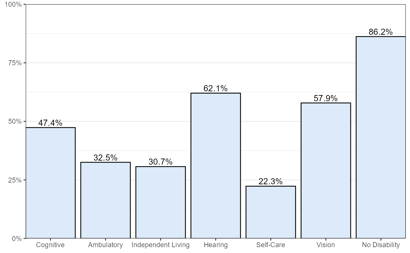
Same information as above, but for all Iowans 16+ years old by Sex
Data was pulled from https://usa.ipums.org/usa/sda/ 2015-2019 5-year ACS. #### Disability variable codes: diffrem:Cognitive difficulty diffphys: Ambulatory difficulty diffmob: Independent living difficulty diffcare: Self-care difficulty diffeye: Vision difficulty diffhear: Hearing difficulty #### Employment variable code: empstat: Employment status #### Sex variable code: sex: Sex
disBySex <- read_csv("../data_raw/sex_disability_employment.csv")
#>
#> -- Column specification --------------------------------------------------------
#> cols(
#>   freq_dist = col_character(),
#>   status = col_character(),
#>   no_dis = col_double(),
#>   yes_dis = col_double(),
#>   row_total = col_double(),
#>   Difficulty = col_character(),
#>   sex = col_character()
#> )
gen <- read_csv("../data_raw/emp_sex.csv")
#>
#> -- Column specification --------------------------------------------------------
#> cols(
#>   freq_dist = col_character(),
#>   Status = col_character(),
#>   `1 Male` = col_double(),
#>   `2 Female` = col_double(),
#>   `ROW TOTAL` = col_double()
#> )
clean_disBySex <- disBySex %>%
  filter(freq_dist=="Weighted N") %>%
  mutate(status=str_remove(status, pattern="\\d"),
         estimate=yes_dis) %>%
  select(-no_dis, -yes_dis, -row_total) %>%
  spread(status, estimate) %>%
  janitor::clean_names() %>%
  mutate(sum = employed + not_in_labor_force + unemployed,
         p_out = not_in_labor_force / sum,
         p_em = employed / sum,
         p_un = unemployed / sum)

clean_gen <- gen %>%
  filter(freq_dist=="Weighted N") %>%
  janitor::clean_names() %>%
  mutate(status=str_remove(status, pattern="\\d"),
         male=x1_male,
         female=x2_female) %>%
  select(-x1_male, -x2_female, -row_total)
clean_gen_male <- clean_gen %>% select (-female) %>%
  spread(status, male) %>%
  mutate(sex="male")
clean_gen_female <- clean_gen %>% select (-male) %>%
  spread(status, female) %>%
  mutate(sex="female")

cleaner_gen <- rbind(clean_gen_male, clean_gen_female) %>%
  janitor::clean_names() %>%
  mutate(sum = employed + not_in_labor_force + unemployed,
         p_out = not_in_labor_force / sum,
         p_em = employed / sum,
         p_un = unemployed / sum,
         difficulty = "overall population")

comb <- rbind(clean_disBySex, cleaner_gen)
comb %>%
  mutate(sex = ifelse(sex == "female","Female","Male"),
         p_out_text = paste0(round(p_out,3)*100,"%"),
         difficulty = factor(difficulty,
                             levels = c("overall population","Ambulatory","cognitive","hearing","independent living","self-care","Vision"),
                             labels = c("Total Pop.","Ambulatory","Cognitive","Hearing","Indep. Living","Self-Care","Vision"))) %>%
  ggplot(aes(x=difficulty, y=p_out, fill=sex)) +
  geom_col(position="dodge")+
  labs(
    x="Difficulty Type",
    fill = "Sex"
  ) +
  theme_bw() +
  scale_fill_manual(values=c("#D81E3F","#2A6EBB")) +
  theme(text = element_text(family = "sans"),
        panel.background = element_rect(fill="white"),
        panel.grid.major.x = element_blank(),
        panel.grid.minor.x = element_blank(),
        panel.grid.minor.y = element_blank(),
        legend.position="top",
        axis.title.y = element_blank(),
        legend.background = element_rect(fill = NA)) +
  geom_text(aes(label = p_out_text), position = position_dodge(0.9), vjust = 1.1, size=4.5, color="white") +
  scale_y_continuous(labels = scales::percent,limits = c(0,1.01)) +
  coord_cartesian(ylim = c(0,1.01),expand = FALSE)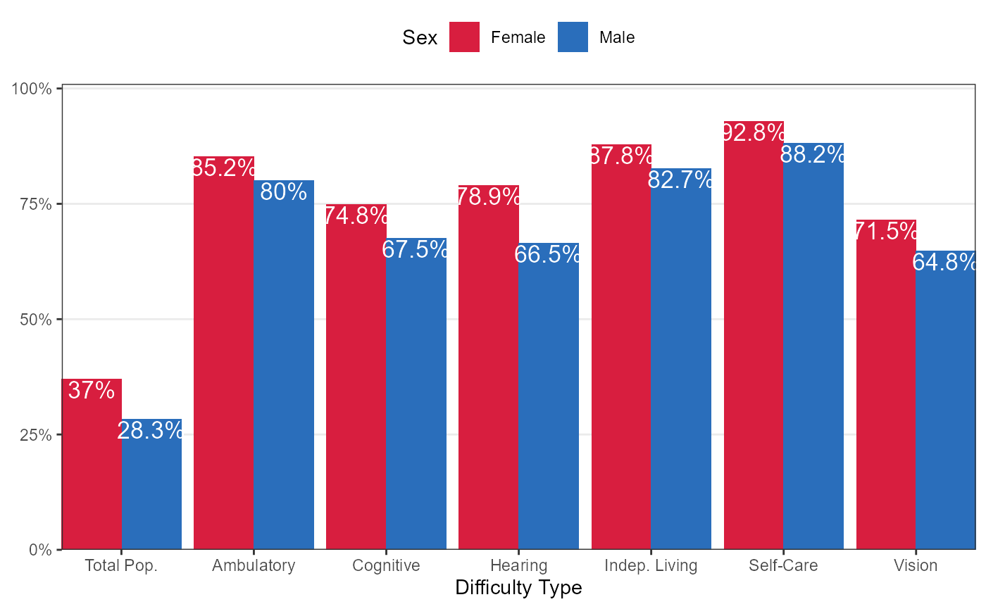
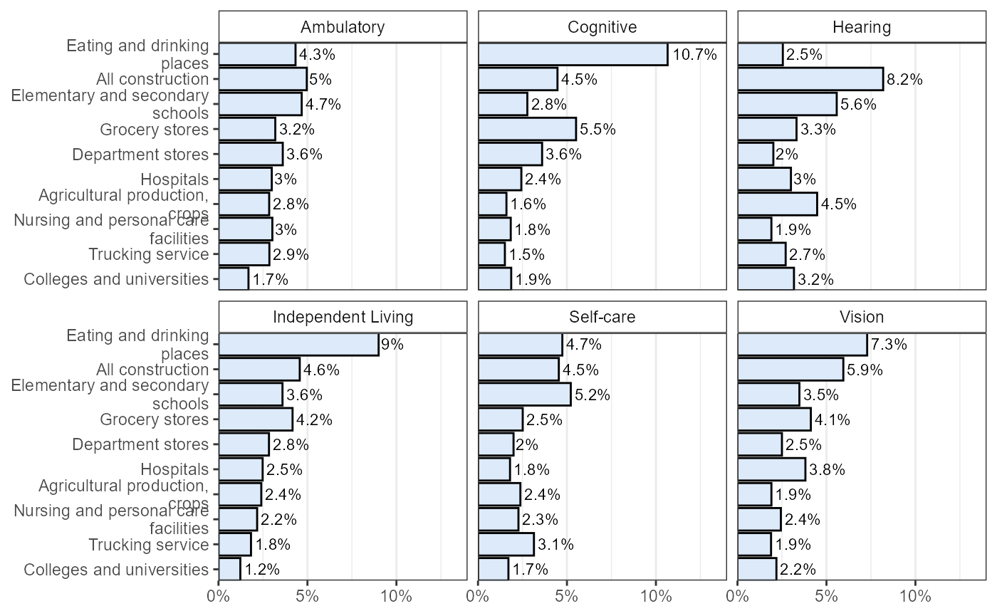
Percentage of Individuals by Disability Type Who Work in Iowa’s Top 10 Industries Ranked by Overall Number of Employees with Disabilities
Same variable codes for disability, industry variable code is IND1990. IND1990 classifies industries from all years since 1950 into the 1990 Census Bureau industrial classification scheme.
hearing <- read_csv("../data_raw/diffhear_ind1990.csv")
#>
#> -- Column specification --------------------------------------------------------
#> cols(
#>   `Frequency Distribution` = col_character(),
#>   Occupation = col_character(),
#>   `1 No` = col_double(),
#>   `2 Yes` = col_double(),
#>   `ROW TOTAL` = col_double()
#> )
cognitive <- read_csv("../data_raw/diffrem_ind1990.csv")
#>
#> -- Column specification --------------------------------------------------------
#> cols(
#>   `Frequency Distribution` = col_character(),
#>   Occupation = col_character(),
#>   `1 No cognitive difficulty` = col_double(),
#>   `2 Has cognitive difficulty` = col_double(),
#>   `ROW TOTAL` = col_double()
#> )
vision <- read_csv("../data_raw/diffeye_ind1990.csv")
#>
#> -- Column specification --------------------------------------------------------
#> cols(
#>   `Frequency Distribution` = col_character(),
#>   Occupation = col_character(),
#>   `1 No` = col_double(),
#>   `2 Yes` = col_double(),
#>   `ROW TOTAL` = col_double()
#> )
ambulatory <- read_csv("../data_raw/diffphys_ind1990.csv")
#>
#> -- Column specification --------------------------------------------------------
#> cols(
#>   `Frequency Distribution` = col_character(),
#>   Occupation = col_character(),
#>   `1 No ambulatory difficulty` = col_double(),
#>   `2 Has ambulatory difficulty` = col_double(),
#>   `ROW TOTAL` = col_double()
#> )
independent <- read_csv("../data_raw/diffmob_ind1990.csv")
#>
#> -- Column specification --------------------------------------------------------
#> cols(
#>   `Frequency Distribution` = col_character(),
#>   Occupation = col_character(),
#>   `1 No independent living difficulty` = col_double(),
#>   `2 Has independent living difficulty` = col_double(),
#>   `ROW TOTAL` = col_double()
#> )
self <- read_csv("../data_raw/diffcare_ind1990.csv")
#>
#> -- Column specification --------------------------------------------------------
#> cols(
#>   `Frequency Distribution` = col_character(),
#>   Occupation = col_character(),
#>   `1 No` = col_double(),
#>   `2 Yes` = col_double(),
#>   `ROW TOTAL` = col_double()
#> )
clean_hearing <- hearing %>%
  janitor::clean_names() %>%
  mutate(
    occ_code = str_extract(occupation, "[:digit:]*"),
    occ_label = str_remove(occupation, occ_code),
    disability = "Hearing difficulty",
    estimate = x2_yes
  ) %>%
  filter(frequency_distribution=="Weighted N") %>%
  select(-x1_no, -row_total, -x2_yes)

clean_self <- self %>%
  janitor::clean_names() %>%
  mutate(
    occ_code = str_extract(occupation, "[:digit:]*"),
    occ_label = str_remove(occupation, occ_code),
    disability = "Self-care difficulty",
    estimate = x2_yes
  ) %>%
  filter(frequency_distribution=="Weighted N") %>%
  select(-x1_no, -row_total, -x2_yes)

clean_cognitive <- cognitive %>%
  janitor::clean_names() %>%
  mutate(
    occ_code = str_extract(occupation, "[:digit:]*"),
    occ_label = str_remove(occupation, occ_code),
    disability = "Cognitive difficulty",
    estimate = x2_has_cognitive_difficulty
  ) %>%
  filter(frequency_distribution=="Weighted N") %>%
  select(-x1_no_cognitive_difficulty, -row_total, -x2_has_cognitive_difficulty)

clean_vision <- vision %>%
  janitor::clean_names() %>%
  mutate(
    occ_code = str_extract(occupation, "[:digit:]*"),
    occ_label = str_remove(occupation, occ_code),
    disability = "Vision difficulty",
    estimate = x2_yes
  ) %>%
  filter(frequency_distribution=="Weighted N") %>%
  select(-x1_no, -row_total, -x2_yes)

clean_ambulatory <- ambulatory %>%
  janitor::clean_names() %>%
  mutate(
    occ_code = str_extract(occupation, "[:digit:]*"),
    occ_label = str_remove(occupation, occ_code),
    disability = "Ambulatory difficulty",
    estimate = x2_has_ambulatory_difficulty
  ) %>%
  filter(frequency_distribution=="Weighted N") %>%
  select(-x1_no_ambulatory_difficulty, -row_total, -x2_has_ambulatory_difficulty)

clean_independent <- independent %>%
  janitor::clean_names() %>%
  mutate(
    occ_code = str_extract(occupation, "[:digit:]*"),
    occ_label = str_remove(occupation, occ_code),
    disability = "Independent living difficulty",
    estimate = x2_has_independent_living_difficulty
  ) %>%
  filter(frequency_distribution=="Weighted N") %>%
  select(-x1_no_independent_living_difficulty, -row_total, -x2_has_independent_living_difficulty)

disability <- rbind(clean_hearing, clean_cognitive, clean_vision, clean_ambulatory, clean_independent, clean_self) %>%
  filter(occ_code != 0, occ_code != 992)

type_totals <- disability %>%
  group_by(disability) %>%
  summarize(dis_total = sum(estimate))

occ_totals <- disability %>%
  group_by(occupation) %>%
  summarize(occ_total = sum(estimate))%>%
  top_n(10, occ_total)

disability <- disability %>%
  right_join(occ_totals, by="occupation") %>%
  left_join(type_totals, by="disability") %>%
  mutate(estimateProp = estimate/dis_total)
disability %>%
  mutate(disability = str_remove(disability," difficulty")) %>%
  mutate(disability = ifelse(disability == "Independent living","Independent Living",disability)) %>%
  ggplot(aes(reorder(occ_label, occ_total), estimateProp)) +
  geom_col(fill="#ddeaf9", colour = "black") +
  facet_wrap(~ disability) +
  geom_text(aes(label = paste0(round(as.numeric(estimateProp*100), 1), "%")),
            hjust = -0.1, size=3, position=position_dodge(0.9)) +
  coord_flip(expand = FALSE) +
  scale_y_continuous(breaks = c(0,.05,.10,.15),
                     labels = c("0%","5%","10%","15%"),
                     limits=c(0, .14)) +
  scale_x_discrete(labels = function(x) stringr::str_wrap(x,width = 25)) +
  theme_bw() +
  theme(text = element_text(family = "sans"),
        panel.grid.major.y = element_blank(),
        panel.background = element_rect(fill = "white"),
        plot.background = element_rect(fill = "white"),
        strip.background = element_rect(fill = "white"),
        axis.title = element_blank())