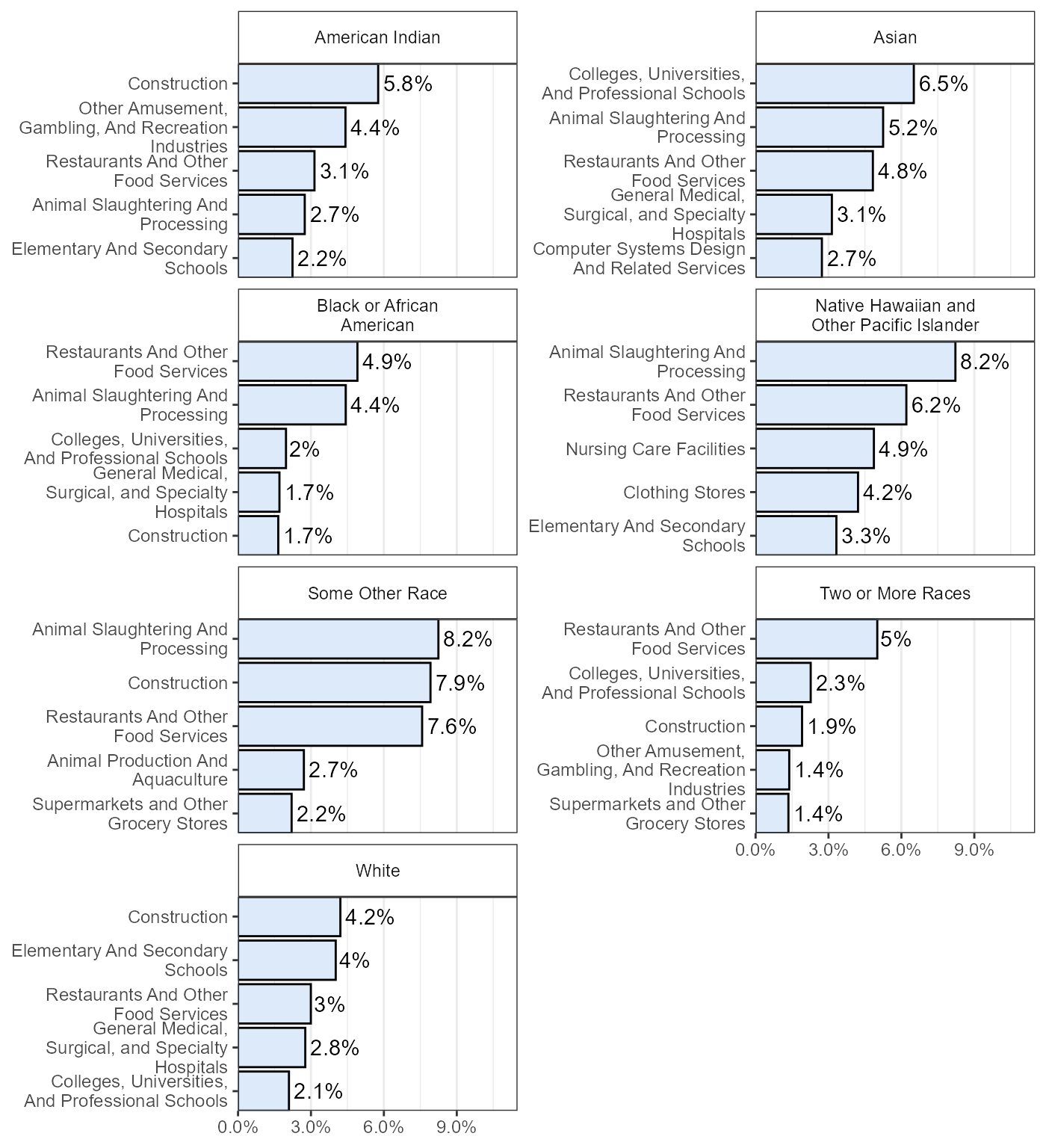
Where are Immigrants and Racial/Ethnic Minorities Working in Iowa?

This is a supplementary vignette for the DHR Workforce Poster “Where are Migrants and Racial/Ethnic Minorities Working in Iowa?”

Recent immigrants and Racial/Ethnic minorities face many economic barriers in the United States. Understanding where these individuals work may help better identify and diminish these barriers.

Top Industries for Workers Moving from Other Countries to Iowa Within the Past Year

We explain any caveats attached the data used to create this poster. For example, if the data originate from a year other than the current year or if we filter-out certain rows based on some criteria (estimates too small, etc.)

library(tidyverse)
# download data set from PUMS
# indByMig <- tidycensus::get_pums(variables = c("INDP","MIGSP"),state = "IA",recode = TRUE)

# data set also saved to the work repo
load("../data_raw/industry_by_migrancyStatus.RData")

indByMig %>%
  mutate(usFlag = ifelse(str_detect(MIGSP_label,"/"),TRUE,FALSE)) %>%
  filter(!usFlag) %>%
  group_by(INDP_label) %>%
  summarise(estimate = sum(PWGTP)) %>%
  mutate(INDP_label = as.character(INDP_label)) %>%
  filter(!is.na(INDP_label)) %>%
  arrange(desc(estimate)) %>%
  rename(industry = INDP_label) %>%
  mutate(industry = str_remove(industry,"^[A-Z]{3}\\-")) %>%
  mutate(industry = str_replace(str_remove(str_remove(industry,"\\(.*\\)"),", Including Junior Colleges"),
                                "General Medical And Surgical Hospitals, And Specialty  Hospitals",
                                "General Medical, Surgical, and Specialty Hospitals")) %>%
  # filter(estimate  > 100) %>%
  top_n(n = 10,wt = estimate) %>%
  ggplot(aes(x = reorder(industry,estimate),y = estimate)) +
  geom_bar(stat = "identity",fill="#ddeaf9", colour = "black") +
  geom_text(aes(label = estimate),hjust = -.12) +
  coord_flip(expand = FALSE) +
  theme_bw() +
  theme(axis.title = element_blank(),
        panel.grid.major.y = element_blank()) +
  scale_x_discrete(labels = function(x) stringr::str_wrap(x,width = 25)) +
  scale_y_continuous(limits = c(0,1300))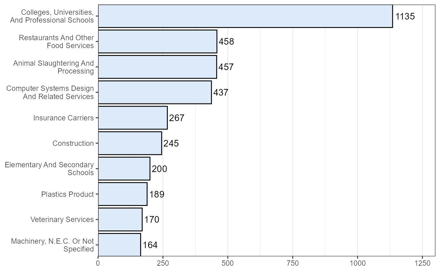

Percentage of Recent Migrants and All Workers Identifying as Hispanic, by Industry

Note that we are including only industries with an estimated number of workforce greater than 100.

# download data set from PUMS
# indByMigbyHispanic <- tidycensus::get_pums(variables = c("HISP","INDP","MIGSP"),state = "IA",year = 2019,survey = "acs5",recode = TRUE)

# or load the data set from the work repo
load( "../data_raw/industry_by_migrancyStatus_hispIdentity.RData")

recentMigrants_indByHispanic <- indByMigbyHispanic %>%
  mutate(usFlag = ifelse(str_detect(MIGSP_label,"/"),TRUE,FALSE)) %>%
  filter(!usFlag) %>%
  mutate(HISP_label = as.character(HISP_label))%>%
  mutate(hisp = ifelse(as.character(HISP_label) == "Not Spanish/Hispanic/Latino",FALSE,TRUE)) %>%
  group_by(hisp,INDP_label) %>%
  summarise(estimate = sum(PWGTP),
            .groups = "drop") %>%
  group_by(INDP_label) %>%
  mutate(total = sum(estimate)) %>%
  filter(hisp & total > 100) %>%
  summarise(propHisp = estimate/total) %>%
  arrange(desc(propHisp)) %>%
  rename(industry = INDP_label) %>%
  mutate(industry = str_remove(industry,"^[A-Z]{3}\\-")) %>%
  mutate(industry = str_replace(str_remove(str_remove(industry,"\\(.*\\)"),", Including Junior Colleges"),
                                "General Medical And Surgical Hospitals, And Specialty  Hospitals",
                                "General Medical, Surgical, and Specialty Hospitals")) %>%
  filter(!is.na(industry)) %>%
  top_n(n = 10,wt = propHisp) %>%
  mutate(migrancy = "Recent Migrants") %>%
  mutate(industry = reorder(industry,propHisp))

recentMigrants_indByHispanic %>%
  mutate(migrancy = factor(migrancy,levels = c("Recent Migrants","All Workers"))) %>%
  ggplot(aes(x = industry,y = propHisp)) +
  geom_bar(stat = "identity",fill = "#fbc6c6ff",colour = "black") +
  geom_text(aes(label = paste0(round(propHisp,3)*100,"%")),
            hjust = -.1) +
  coord_flip(expand = FALSE,ylim = c(0,1.08)) +
  scale_x_discrete(labels = function(x) str_wrap(x,width = 25)) +
  scale_y_continuous(labels = scales::percent) +
  theme_bw() +
  theme(axis.title = element_blank(),
        panel.grid.major.y = element_blank(),
        legend.position = "none")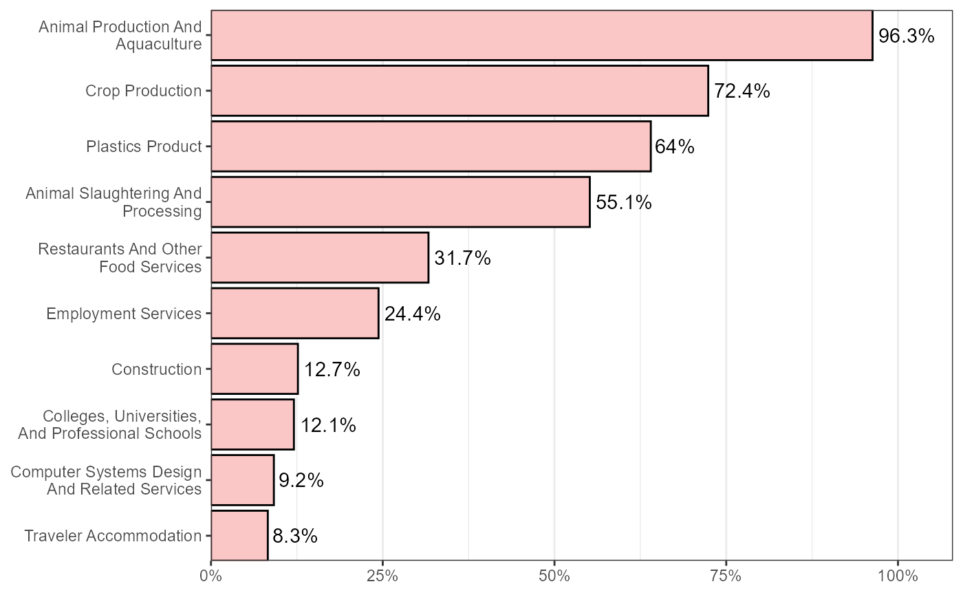

Add Hispanic-identifying percentages for all Iowa workers to plot above

allWorkers_indByHispanic <- indByMigbyHispanic %>%
  mutate(HISP_label = as.character(HISP_label))%>%
  mutate(hisp = ifelse(as.character(HISP_label) == "Not Spanish/Hispanic/Latino",FALSE,TRUE)) %>%
  group_by(hisp,INDP_label) %>%
  summarise(estimate = sum(PWGTP),
            .groups = "drop") %>%
  group_by(INDP_label) %>%
  mutate(total = sum(estimate)) %>%
  filter(hisp & total > 100) %>%
  summarise(propHisp = estimate/total) %>%
  arrange(desc(propHisp)) %>%
  rename(industry = INDP_label) %>%
  mutate(industry = str_remove(industry,"^[A-Z]{3}\\-")) %>%
  mutate(industry = str_replace(str_remove(str_remove(industry,"\\(.*\\)"),", Including Junior Colleges"),
                                "General Medical And Surgical Hospitals, And Specialty  Hospitals",
                                "General Medical, Surgical, and Specialty Hospitals")) %>%
  filter(industry %in% recentMigrants_indByHispanic$industry) %>%
  mutate(migrancy = "All Workers",
         industry = factor(industry,levels = levels(recentMigrants_indByHispanic$industry)))

bind_rows(recentMigrants_indByHispanic,
                 allWorkers_indByHispanic) %>%
  mutate(migrancy = factor(migrancy,levels = c("Recent Migrants","All Workers"))) %>%
  ggplot(aes(x = industry,y = propHisp)) +
  geom_bar(stat = "identity",aes(fill = migrancy),colour = "black") +
  geom_text(aes(label = paste0(round(propHisp,3)*100,"%")),
            hjust = -.1) +
  coord_flip(expand = FALSE,ylim = c(0,1.2)) +
  scale_x_discrete(labels = function(x) str_wrap(x,width = 25)) +
  scale_y_continuous(labels = scales::percent) +
  theme_bw() +
  theme(axis.title = element_blank(),
        panel.grid.major.y = element_blank()) +
  facet_wrap(~ migrancy,ncol = 2) +
  scale_fill_manual(values = c("#2A6EBB","#D81E3F"))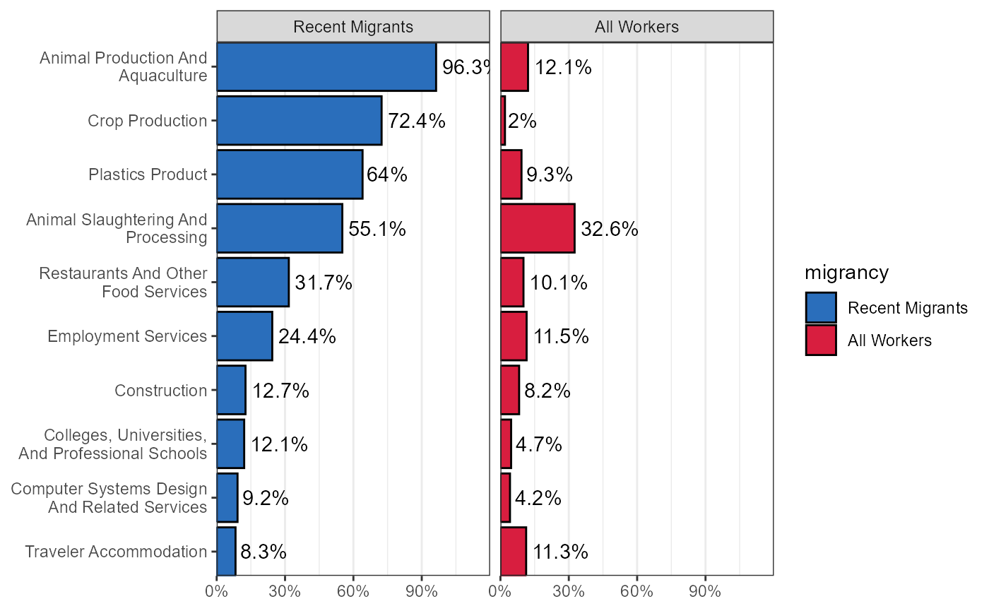

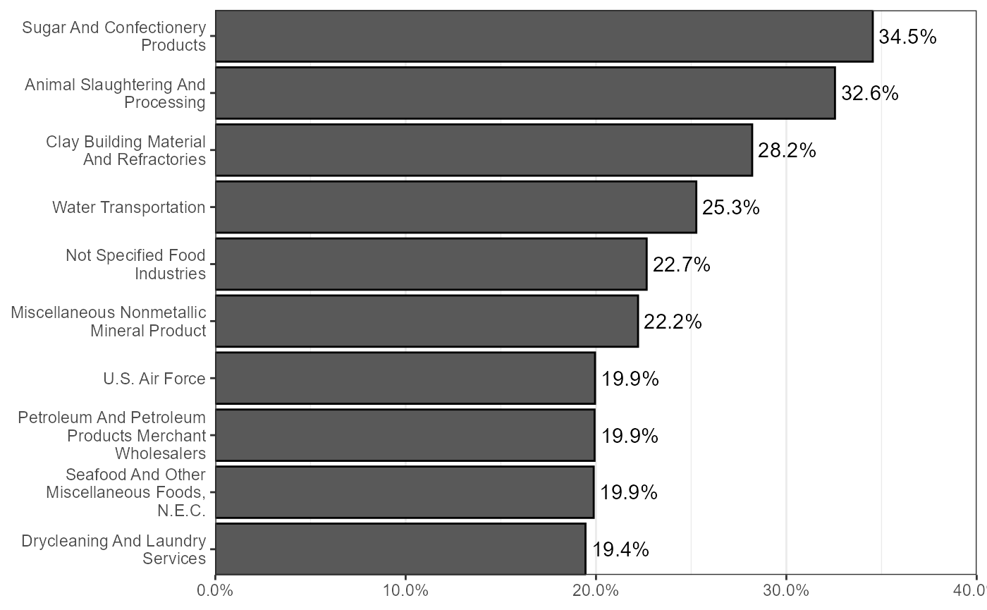
Top industries for all Iowa workers identifying as Hispanic

indByMigbyHispanic %>%
  mutate(HISP_label = as.character(HISP_label))%>%
  mutate(hisp = ifelse(as.character(HISP_label) == "Not Spanish/Hispanic/Latino",FALSE,TRUE)) %>%
  group_by(hisp,INDP_label) %>%
  summarise(estimate = sum(PWGTP),
            .groups = "drop") %>%
  group_by(INDP_label) %>%
  mutate(total = sum(estimate)) %>%
  filter(hisp & total > 100) %>%
  summarise(propHisp = estimate/total) %>%
  arrange(desc(propHisp)) %>%
  rename(industry = INDP_label) %>%
  mutate(industry = str_remove(industry,"^[A-Z]{3}\\-")) %>%
  mutate(industry = str_replace(str_remove(str_remove(industry,"\\(.*\\)"),", Including Junior Colleges"),
                                "General Medical And Surgical Hospitals, And Specialty  Hospitals",
                                "General Medical, Surgical, and Specialty Hospitals")) %>%
  top_n(n = 10,wt = propHisp)  %>%
  ggplot(aes(x = reorder(industry,propHisp),y = propHisp)) +
  geom_bar(stat = "identity",colour = "black") +
  geom_text(aes(label = paste0(round(propHisp,3)*100,"%")),
            hjust = -.1) +
  coord_flip(expand = FALSE,ylim = c(0,.4)) +
  scale_x_discrete(labels = function(x) str_wrap(x,width = 25)) +
  scale_y_continuous(labels = scales::percent) +
  theme_bw() +
  theme(axis.title = element_blank(),
        panel.grid.major.y = element_blank(),
        legend.position = "none")

Top 5 Industries by Their Percentage Share of All Workers in the Race Group

Note that we we do not include the categories of “Alaska Native alone” or “American Indian and Alaska Native tribes specified; or American Indian or Alaska Native, not specified and no other races” due to relatively small (unreliable) estimates.

# download data from PUMS
# industryByRace <- tidycensus::get_pums(variables = c("INDP","RAC1P"),state = "IA",recode = TRUE)

# or load the data set from the work repo
load("../data_raw/topIndustries_by_Race.RData")

industryByRace %>%
  group_by(INDP_label,RAC1P_label) %>%
  summarise(estimate = sum(PWGTP)) %>%
  rename(industry = INDP_label,
         race = RAC1P_label) %>%
  mutate(industry = as.character(industry),
         race = as.character(race)) %>%
  group_by(race) %>%
  arrange(race,desc(estimate)) %>%
  mutate(total = sum(estimate)) %>%
  filter(!is.na(industry)) %>%
  top_n(n = 5,wt = estimate) %>%
  mutate(industry = str_remove(industry,"^[A-Z]{3}\\-")) %>%
  mutate(prop = estimate/total)  %>%
  filter(!(race %in% c("Alaska Native alone","American Indian and Alaska Native tribes specified; or American Indian or Alaska Native, not specified and no other races"))) %>%
  mutate(industry = str_replace(str_remove(str_remove(industry,"\\(.*\\)"),", Including Junior Colleges"),
                                "General Medical And Surgical Hospitals, And Specialty  Hospitals",
                                "General Medical, Surgical, and Specialty Hospitals")) %>%
  mutate(industry = tidytext::reorder_within(industry,prop,race)) %>%
  mutate(race = str_remove(str_remove(race," alone")," tribes specified; or American Indian or Alaska Native, not specified and no other races")) %>%
  ggplot(aes(x = industry,y = prop)) +
  geom_bar(stat = "identity",fill="#ddeaf9", colour = "black") +
  geom_text(aes(label = paste0(round(prop,3)*100,"%")),
            hjust = -.1) +
  facet_wrap(~ race,scales = "free_y",ncol = 2,
             labeller = labeller(race = label_wrap_gen(25))) +
  theme_bw() +
  theme(axis.text = element_text(size = 9),
        axis.title = element_blank(),
        strip.background = element_rect(fill = NA),
        panel.grid.major.y = element_blank()) +
  coord_flip(expand = FALSE) +
  scale_y_continuous(limits = c(0,.115),
                     labels = scales::percent) +
  scale_x_discrete(labels = function(x) stringr::str_wrap(stringr::str_remove(x,"___.*"),width = 25))
#> `summarise()` has grouped output by 'INDP_label'. You can override using the `.groups` argument.