How Do Race, Ethnicity, and Disability Status Affect how Iowans Commute to Work?
commuteByRaceEthnicityDisability.RmdThis is a supplementary vignette for the DHR Workforce Poster “How Do Race, Ethnicity, and Disability Status Affect how Iowans Commute to Work?”
Lack of access to adequate means of transportation to work is a significant barrier to full participation in the workforce. This poster combines data from the American Community Survey (ACS) and Public-Use Microdata Samples (PUMS) to examine differences in commuting times and methods by race and disability status.
Time Spent Commuting to Work by Race
PUMS data is loaded and cleaned. When downloading PUMS data (trantime by race), filters “statefip(19)” and “empstat(1)” were used to select the desired population (employed Iowans). Please note that two aggregations were performed - Chinese, Japanese, and Other Asian or Pacific Islander were aggregated into Asian or Pacific Islander and Two Major Races and Three or More Major Races were aggregated into Two or Mores Races.
library(tidyverse)

commute_time_by_race <- data.frame(read.csv("../data_clean/commute_time_by_race.csv"))

cleaned_commute_race <- commute_time_by_race %>%
  filter(X == "Weighted N") %>%
  mutate(Asian.or.Pacific.Islander = Chinese + Japanese + Other.Asian.or.Pacific.Islander) %>%
  mutate(Two.or.More.Races = Two.major.races + Three.or.more.major.races) %>%
  select(-Chinese, -Japanese, -Other.Asian.or.Pacific.Islander, -Two.major.races, -Three.or.more.major.races, ROW.TOTAL) %>%
  filter(X.1 != "COL TOTAL") %>%
  pivot_longer(White:ncol(.)) %>%
  group_by(name) %>%
  mutate(percent = 100*value/sum(value)) %>%
  mutate(name = ifelse(name == "Black.African.American", "Black or African American", name)) %>%
  mutate(name = ifelse(name == "American.Indian.or.Alaska.Native", "American Indian or Alaska Native", name)) %>%
  mutate(name = ifelse(name == "Other.race..nec", "Other", name)) %>%
  mutate(name = ifelse(name == "ROW.TOTAL", "All Races", name)) %>%
  mutate(name = ifelse(name == "Asian.or.Pacific.Islander", "Asian or Pacific Islander", name)) %>%
  mutate(name = ifelse(name == "Two.or.More.Races", "Two or More Races", name))

ylabord <- c("0-9", "10-19", "20-29", "30-39", "40-49", "50-59", "60+")

cleaned_commute_race <- cleaned_commute_race %>%
  mutate(X.1 = ifelse(X.1 == "120+", "100+", X.1)) %>%
  mutate(X.1 = ifelse(X.1 %in% c("60-69", "70-79", "80-89", "90-99", "100+"),"60+",X.1)) %>%
  mutate(X.1 = factor(X.1, levels = ylabord)) %>%
  mutate(name = factor(name, levels = c("American Indian or Alaska Native", "Asian", "Black or African American", "Asian or Pacific Islander", "White", "Two or More Races", "Other", "All Races")))
Data is plotted to show commute times by race.
cleaned_commute_race %>%
  group_by(name) %>%
  mutate(total = sum(value)) %>%
  group_by(name,X.1) %>%
  summarise(value = sum(value)/total) %>%
  distinct() %>%
  ggplot(aes(x = X.1, y = value)) +
  geom_bar(stat = "identity", fill = "#C41230",colour = "black") +
  facet_wrap(~name, nrow = 2,labeller = labeller(name = label_wrap_gen(25))) +
  coord_flip(expand = FALSE) +
  theme_bw() +
  scale_y_continuous(labels = function(x) str_remove(scales::percent(x),"\\.0")) +
  theme(legend.position = "none",
        axis.title = element_blank(),
        axis.text = element_text(size = 11),
        strip.text = element_text(size = 11),
        panel.grid.major.y = element_blank(),
        strip.background = element_rect(fill = NA))
#> `summarise()` has grouped output by 'name', 'X.1'. You can override using the `.groups` argument.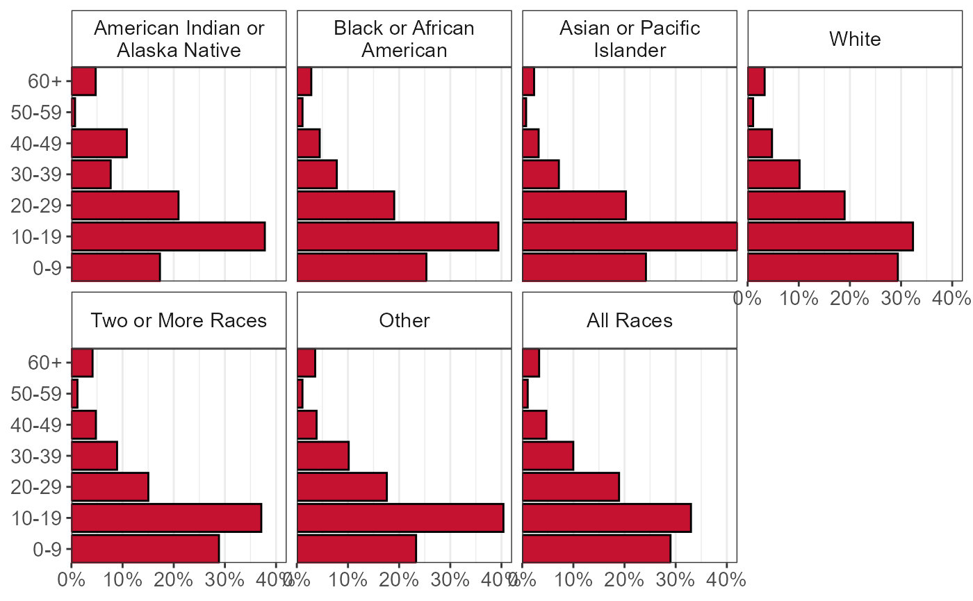
Percent of Workforce Driving Alone to Work by Race
Download transportation by race data from ACS for commute methods of interest.
# download data from ACS
statewide_commute_white <- get_acs(geography = "state",
                                   state = "IA",
                                   variables = c(drove_alone = "B08105A_002", carpooled = "B08105A_003", public_transit = "B08105A_004", walked = "B08105A_005")
) %>%
  rename("est_pop" = estimate, "moe_pop" = moe) %>%
  mutate(race = "White") %>%
  mutate(percent_of_pop = est_pop / sum(est_pop))

statewide_commute_black <- get_acs(geography = "state",
                                   state = "IA",
                                   variables = c(drove_alone = "B08105B_002", carpooled = "B08105B_003", public_transit = "B08105B_004", walked = "B08105B_005")
) %>%
  rename("est_pop" = estimate, "moe_pop" = moe) %>%
  mutate(race = "Black") %>%
  mutate(percent_of_pop = est_pop / sum(est_pop))

statewide_commute_native <- get_acs(geography = "state",
                                    state = "IA",
                                    variables = c(drove_alone = "B08105C_002", carpooled = "B08105C_003", public_transit = "B08105C_004", walked = "B08105C_005")
) %>%
  rename("est_pop" = estimate, "moe_pop" = moe) %>%
  mutate(race = "American Indian and Alaska Native") %>%
  mutate(percent_of_pop = est_pop / sum(est_pop))

statewide_commute_asian <- get_acs(geography = "state",
                                   state = "IA",
                                   variables = c(drove_alone = "B08105D_002", carpooled = "B08105D_003", public_transit = "B08105D_004", walked = "B08105D_005")
) %>%
  rename("est_pop" = estimate, "moe_pop" = moe) %>%
  mutate(race = "Asian") %>%
  mutate(percent_of_pop = est_pop / sum(est_pop))

statewide_commute_pacific <- get_acs(geography = "state",
                                     state = "IA",
                                     variables = c(drove_alone = "B08105E_002", carpooled = "B08105E_003", public_transit = "B08105E_004", walked = "B08105E_005")
) %>%
  rename("est_pop" = estimate, "moe_pop" = moe) %>%
  mutate(race = "Native Hawaiian and Other Pacific Islander") %>%
  mutate(percent_of_pop = est_pop / sum(est_pop))

statewide_commute_other <- get_acs(geography = "state",
                                   state = "IA",
                                   variables = c(drove_alone = "B08105F_002", carpooled = "B08105F_003", public_transit = "B08105F_004", walked = "B08105F_005")
) %>%
  rename("est_pop" = estimate, "moe_pop" = moe) %>%
  mutate(race = "Other") %>%
  mutate(percent_of_pop = est_pop / sum(est_pop))

statewide_commute_two <- get_acs(geography = "state",
                                 state = "IA",
                                 variables = c(drove_alone = "B08105G_002", carpooled = "B08105G_003", public_transit = "B08105G_004", walked = "B08105G_005")
) %>%
  rename("est_pop" = estimate, "moe_pop" = moe) %>%
  mutate(race = "Two or More") %>%
  mutate(percent_of_pop = est_pop / sum(est_pop))

statewide_commute_hispanic <- get_acs(geography = "state",
                                      state = "IA",
                                      variables = c(drove_alone = "B08105I_002", carpooled = "B08105I_003", public_transit = "B08105I_004", walked = "B08105I_005")
) %>%
  rename("est_pop" = estimate, "moe_pop" = moe) %>%
  mutate(race = "Hispanic or Latino") %>%
  mutate(percent_of_pop = est_pop / sum(est_pop))


statewide_commute_all <- rbind(statewide_commute_white, statewide_commute_black, statewide_commute_native,
                               statewide_commute_asian, statewide_commute_pacific, statewide_commute_other,
                               statewide_commute_two, statewide_commute_hispanic) %>%
  mutate(percent_of_pop = 100*percent_of_pop) %>%
  mutate(race = factor(race, levels = c("Black", "White", "American Indian and Alaska Native", "Asian", "Hispanic or Latino", "Native Hawaiian and Other Pacific Islander", "Two or More", "Other")))
A file containing the data of interest can also be found directly in the GitHub repository.
# or load the combined data set from the work repo
load("../data_raw/commuteType_by_race.RData")
Data is plotted to show variations in the percent of each racial group driving alone to work.
statewide_commute_all %>%
  mutate(prop = percent_of_pop/100) %>%
  filter(variable == "drove_alone") %>%
  ggplot(aes(x = race, y = prop)) +
  geom_bar(stat = "identity", fill = "#005DAB",colour = "black") +
  geom_text(aes(label = paste0(round(prop,3)*100,"%")),vjust = -.3) +
  theme_bw() +
  theme(axis.title = element_blank(),
        panel.grid.major.x = element_blank()) +
  coord_cartesian(expand = FALSE,ylim = c(0,1)) +
  scale_y_continuous(labels = scales::percent) +
  scale_x_discrete(labels = function(x) str_wrap(x,width = 15))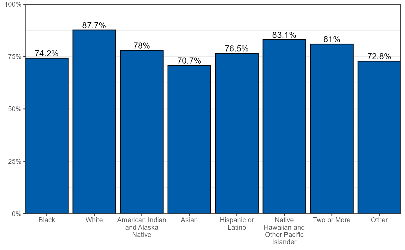
Percent of Households Without Access to a Car by Race
PUMS data is loaded and cleaned. When downloading PUMS data (vehicle by race), the filter “statefip(19)” was used to select the desired population (Iowans). Please note that the same aggregations were made here as in the commute time by race plot.
vehicles_by_race <- data.frame(read.csv(file = "../data_raw/vehiclesByRace.csv"))

cleaned_vehicles_by_race <- vehicles_by_race %>%
  filter(X == "Weighted N") %>%
  mutate(Asian.or.Pacific.Islander = Chinese + Japanese + Other.Asian.or.Pacific.Islander) %>%
  mutate(Two.or.More.Races = Two.major.races + Three.or.more.major.races) %>%
  select(-Chinese, -Japanese, -Other.Asian.or.Pacific.Islander, -Two.major.races, -Three.or.more.major.races, ROW.TOTAL) %>%
  filter(Vehicles.available != "COL TOTAL") %>%
  pivot_longer(White:ncol(.)) %>%
  group_by(name) %>%
  mutate(percent = 100*value/sum(value)) %>%
  mutate(name = ifelse(name == "Black.African.American.Negro", "Black or African American", name)) %>%
  mutate(name = ifelse(name == "American.Indian.or.Alaska.Native", "American Indian or Alaska Native", name)) %>%
  mutate(name = ifelse(name == "Other.race..nec", "Other", name)) %>%
  mutate(name = ifelse(name == "ROW.TOTAL", "All Races", name)) %>%
  mutate(name = ifelse(name == "Asian.or.Pacific.Islander", "Asian or Pacific Islander", name)) %>%
  mutate(name = ifelse(name == "Two.or.More.Races", "Two or More Races", name))

no_vehicle_access <- cleaned_vehicles_by_race %>%
  filter(Vehicles.available == 0)

no_vehicle_access %>%
  mutate(name = factor(name,
                       levels = c("Black or African American","White","American Indian or Alaska Native","Asian or Pacific Islander",
                                  "Two or More Races","Other","All Races"))) %>%
  mutate(prop = percent/100) %>%
  ggplot(aes(x = name, y = prop)) +
  geom_bar(stat = "identity", fill = "#005DAB") +
  geom_text(aes(label = paste0(round(prop,3)*100,"%")),
            vjust = -.3) +
  theme_bw() +
  theme(
    axis.title = element_blank(),
    panel.grid.major.x = element_blank()) +
  coord_cartesian(expand = FALSE,ylim = c(0,.16)) +
  scale_y_continuous(labels = scales::percent) +
  scale_x_discrete(labels = function(x) str_wrap(x,width = 15))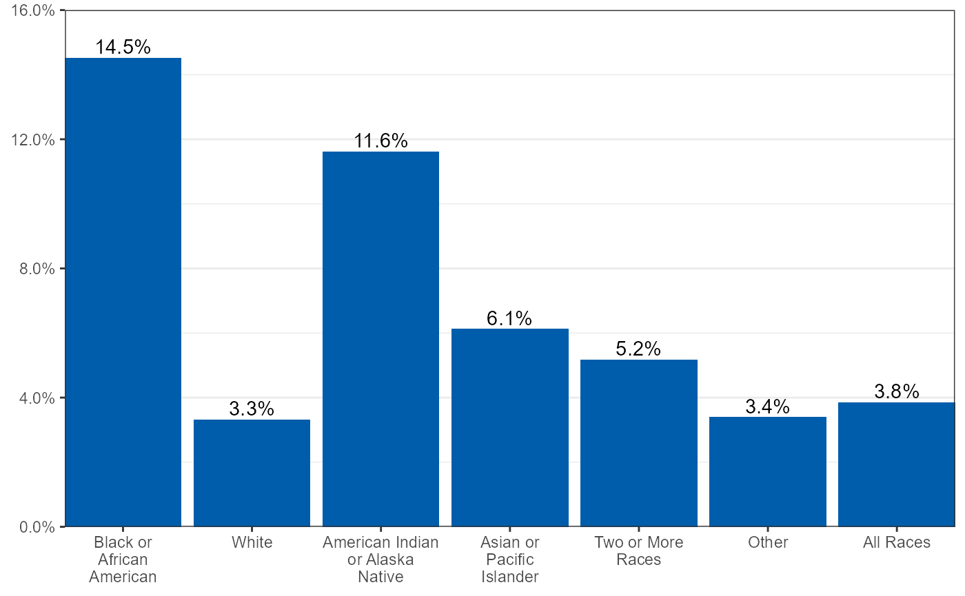
Time Spent Commuting to Work by Disability Status/Type
PUMS data is loaded and cleaned. The first data set (trantime by diffrem, diffphys, diffmob, diffcare, diffsens, diffeye, and diffhear) contains information on commuting times of individuals with various disabilities, with filters “statefip(19)” and “empstat(1)” used to select the desired population (employed Iowans). The second data set (trantime) contains information on commuting times of individuals without disabilities, with filters “statefip(19),” “empstat(1),” and “diffrem(1) diffphys(1) diffmob(1) diffcare(1) diffsens(1) diffeye(1) diffhear(1)” used to select the desired population (employed Iowans with no disabilities).
commute_time_by_disability <- read.csv("../data_raw/disabilityCommuteEmployedFinal.csv")
commute_time_by_noDisability <- read.csv("../data_raw/noDisabilityCommuteEmployedFinal.csv")
commute_time_by_disability %>%
  pivot_longer(3:9,
               names_to = "difficulty",
               values_to = "perc") %>%
  rename(timeGroup = X.1) %>%
  mutate(prop = perc/100,
         difficulty  = str_remove(str_remove(difficulty,"Has\\."),"\\.difficulty")) %>%
  select(timeGroup,difficulty,prop) %>%
  filter(timeGroup != "COL TOTAL") %>%
  mutate(timeGroup = factor(str_remove(timeGroup,"^[0-9]{1} "),
                            levels = c("0-9","10-19","20-29","30-39","40-49","50-59","60+"))) %>%
  bind_rows(commute_time_by_noDisability %>%
              select(Minutes,Percent) %>%
              rename(timeGroup = Minutes) %>%
              mutate(prop = Percent/100,
                     difficulty = "No Disabilities",
                     timeGroup = factor(str_remove(timeGroup,"^[0-9] "),
                                        levels = c("0-9","10-19","20-29","30-39","40-49","50-59","60+"))) %>%
              select(-Percent)) %>%
  mutate(difficulty = factor(str_replace_all(difficulty,"\\."," "),
                             levels = c("ambulatory","cognitive","hearing","independent living","No Disabilities","self care","vision","vision or hearing"),
                             labels = c("Ambulatory","Cognitive","Hearing","Independent Living","No Disabilities","Self-Care","Vision","Vision or Hearing"))) %>%
  arrange(timeGroup,difficulty) %>%
  ggplot(aes(x = timeGroup,y = prop)) +
  geom_bar(stat = "identity",fill = "#005DAB",colour = "black") +
  coord_flip(expand = FALSE) +
  theme_bw() +
  theme(axis.title = element_blank(),
        axis.text = element_text(size = 8),
        panel.grid.major.y  = element_blank(),
        strip.background = element_rect(fill = NA)) +
  facet_wrap(~ difficulty,
             ncol = 4) +
  scale_y_continuous(labels = scales::percent,limits = c(0,.45))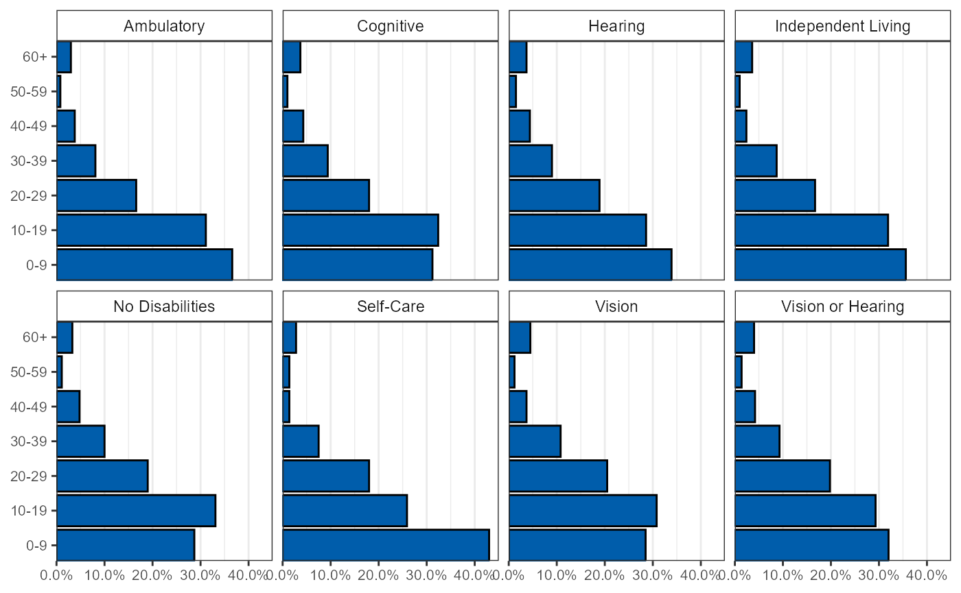
Additional Material
Public Transportation Usage by Race for Black Hawk County
More detailed information about commuting and race in a particular county can be extracted, as shown below with the example of Black Hawk county.
# Download data from ACS

#AMOUNT OF TIME EACH COMMUTE TIME SPENDS GETTING TO WORK BY COUNT // NOT RELATED TO ANY DEMOGRAPHIC
commuteTimeByMode <- get_acs(geography = "county",
                             state = "IA",
                             variables = c(drove_alone = "B08136_003", carpooled = "B08136_004", public_transit = "B08136_007", walked = "B08136_011")
) %>%
  rename("est_time" = estimate, "moe_time" = moe) %>%
  mutate(aggregate_minutes_travelled_per_day = est_time / 7)


# WHITE COMMUTE DATA
commuteModeWhite <- get_acs(geography = "county",
                            state = "IA",
                            variables = c(drove_alone = "B08105A_002", carpooled = "B08105A_003", public_transit = "B08105A_004", walked = "B08105A_005")
) %>%
  rename("est_pop" = estimate, "moe_pop" = moe)

commuteTimeWhite <- left_join(commuteTimeByMode, commuteModeWhite, by = c("GEOID", "NAME", "variable")) %>%
  group_by(NAME) %>%
  mutate(percent_of_pop = est_pop / sum(est_pop)) %>%
  mutate(race = "White")


# BLACK COMMUTE DATA
commuteModeBlack <- get_acs(geography = "county",
                            state = "IA",
                            variables = c(drove_alone = "B08105B_002", carpooled = "B08105B_003", public_transit = "B08105B_004", walked = "B08105B_005")) %>%
  rename("est_pop" = estimate, "moe_pop" = moe)

commuteTimeBlack <- left_join(commuteTimeByMode, commuteModeBlack, by = c("GEOID", "NAME", "variable")) %>%
  group_by(NAME) %>%
  mutate(percent_of_pop = est_pop / sum(est_pop)) %>%
  mutate(race = "Black")


# AMERICAN INDIAN AND ALASKA NATIVE COMMUTE DATA
commuteModeNative <- get_acs(geography = "county",
                             state = "IA",
                             variables = c(drove_alone = "B08105C_002", carpooled = "B08105C_003", public_transit = "B08105C_004", walked = "B08105C_005")) %>%
  rename("est_pop" = estimate, "moe_pop" = moe)

commuteTimeNative <- left_join(commuteTimeByMode, commuteModeNative, by = c("GEOID", "NAME", "variable")) %>%
  group_by(NAME) %>%
  mutate(percent_of_pop = est_pop / sum(est_pop)) %>%
  mutate(race = "Native American")


# ASIAN COMMUTE DATA
commuteModeAsian <- get_acs(geography = "county",
                            state = "IA",
                            variables = c(drove_alone = "B08105D_002", carpooled = "B08105D_003", public_transit = "B08105D_004", walked = "B08105D_005")) %>%
  rename("est_pop" = estimate, "moe_pop" = moe)

commuteTimeAsian <- left_join(commuteTimeByMode, commuteModeAsian, by = c("GEOID", "NAME", "variable")) %>%
  group_by(NAME) %>%
  mutate(percent_of_pop = est_pop / sum(est_pop)) %>%
  mutate(race = "Asian")


# NATIVE HAWAIIAN AND OTHER PACIFIC ISLANDER COMMUTE DATA
commuteModePacific <- get_acs(geography = "county",
                              state = "IA",
                              variables = c(drove_alone = "B08105E_002", carpooled = "B08105E_003", public_transit = "B08105E_004", walked = "B08105E_005")) %>%
  rename("est_pop" = estimate, "moe_pop" = moe)

commuteTimePacific <- left_join(commuteTimeByMode, commuteModePacific, by = c("GEOID", "NAME", "variable")) %>%
  group_by(NAME) %>%
  mutate(percent_of_pop = est_pop / sum(est_pop)) %>%
  mutate(race = "Pacific Islander")


# OTHER RACE COMMUTE DATA
commuteModeOther <- get_acs(geography = "county",
                            state = "IA",
                            variables = c(drove_alone = "B08105F_002", carpooled = "B08105F_003", public_transit = "B08105F_004", walked = "B08105F_005")) %>%
  rename("est_pop" = estimate, "moe_pop" = moe)

commuteTimeOther <- left_join(commuteTimeByMode, commuteModeOther, by = c("GEOID", "NAME", "variable")) %>%
  group_by(NAME) %>%
  mutate(percent_of_pop = est_pop / sum(est_pop)) %>%
  mutate(race = "Other")


# TWO OR MORE RACES COMMUTE DATA
commuteModeTwo <- get_acs(geography = "county",
                          state = "IA",
                          variables = c(drove_alone = "B08105G_002", carpooled = "B08105G_003", public_transit = "B08105G_004", walked = "B08105G_005")) %>%
  rename("est_pop" = estimate, "moe_pop" = moe)

commuteTimeTwo <- left_join(commuteTimeByMode, commuteModeTwo, by = c("GEOID", "NAME", "variable")) %>%
  group_by(NAME) %>%
  mutate(percent_of_pop = est_pop / sum(est_pop)) %>%
  mutate(race = "Two or More")


# HISPANIC AND LATINO COMMUTE DATA
commuteModeHispanic <- get_acs(geography = "county",
                               state = "IA",
                               variables = c(drove_alone = "B08105I_002", carpooled = "B08105I_003", public_transit = "B08105I_004", walked = "B08105I_005")) %>%
  rename("est_pop" = estimate, "moe_pop" = moe)

commuteTimeHispanic <- left_join(commuteTimeByMode, commuteModeHispanic, by = c("GEOID", "NAME", "variable")) %>%
  group_by(NAME) %>%
  mutate(percent_of_pop = est_pop / sum(est_pop)) %>%
  mutate(race = "Hispanic or Latino")


blackHawkAvgWhitePublicTransitPercent <- commuteTimeWhite %>%
  filter(GEOID == 19013, variable == "public_transit") %>%
  mutate(race = "White")

blackHawkAvgBlackPublicTransitPercent <- commuteTimeBlack %>%
  filter(GEOID == 19013, variable == "public_transit") %>%
  mutate(race = "Black")

blackHawkAvgNativePublicTransityPercent <- commuteTimeNative %>%
  filter(GEOID == 19013, variable == "public_transit") %>%
  mutate(race = "Native American")

blackHawkAvgAsianPublicTransitPercent <- commuteTimeAsian %>%
  filter(GEOID == 19013, variable == "public_transit") %>%
  mutate(race = "Asian")

blackHawkAvgPacificPublicTransitPercent <- commuteTimePacific %>%
  filter(GEOID == 19013, variable == "public_transit") %>%
  mutate(race = "Pacific Islander")

blackHawkAvgOtherPublicTransitPercent <- commuteTimeOther %>%
  filter(GEOID == 19013, variable == "public_transit") %>%
  mutate(race = "Other")

blackHawkAvgTwoPublicTransitPercent <- commuteTimeTwo %>%
  filter(GEOID == 19013, variable == "public_transit") %>%
  mutate(race = "Two or More")

blackHawkAvgHispanicPublicTransitPercent <- commuteTimeHispanic %>%
  filter(GEOID == 19013, variable == "public_transit") %>%
  mutate(race = "Hispanic or Latino")

blackHawkCombined <- rbind(blackHawkAvgWhitePublicTransitPercent, blackHawkAvgBlackPublicTransitPercent, blackHawkAvgNativePublicTransityPercent, blackHawkAvgAsianPublicTransitPercent, blackHawkAvgPacificPublicTransitPercent, blackHawkAvgOtherPublicTransitPercent, blackHawkAvgTwoPublicTransitPercent, blackHawkAvgHispanicPublicTransitPercent) %>%
  arrange(desc(percent_of_pop))
# or load from the work repo
load("../data_raw/publicTransitbyRace_blackHawk.RData")
# PERCENT OF EACH RACIAL POPULATION IN BLACK HAWK THAT CARPOOLS TO WORK
ggplot(blackHawkCombined, aes(x = factor(race), y = 100*percent_of_pop)) +
  geom_bar(stat = "identity") +
  labs(title = "% of Workforce Taking Public Transit by Race (BH)", x = "Race", y = "%", subtitle = "2019 5-Year ACS") +
  coord_flip() +
  theme_bw()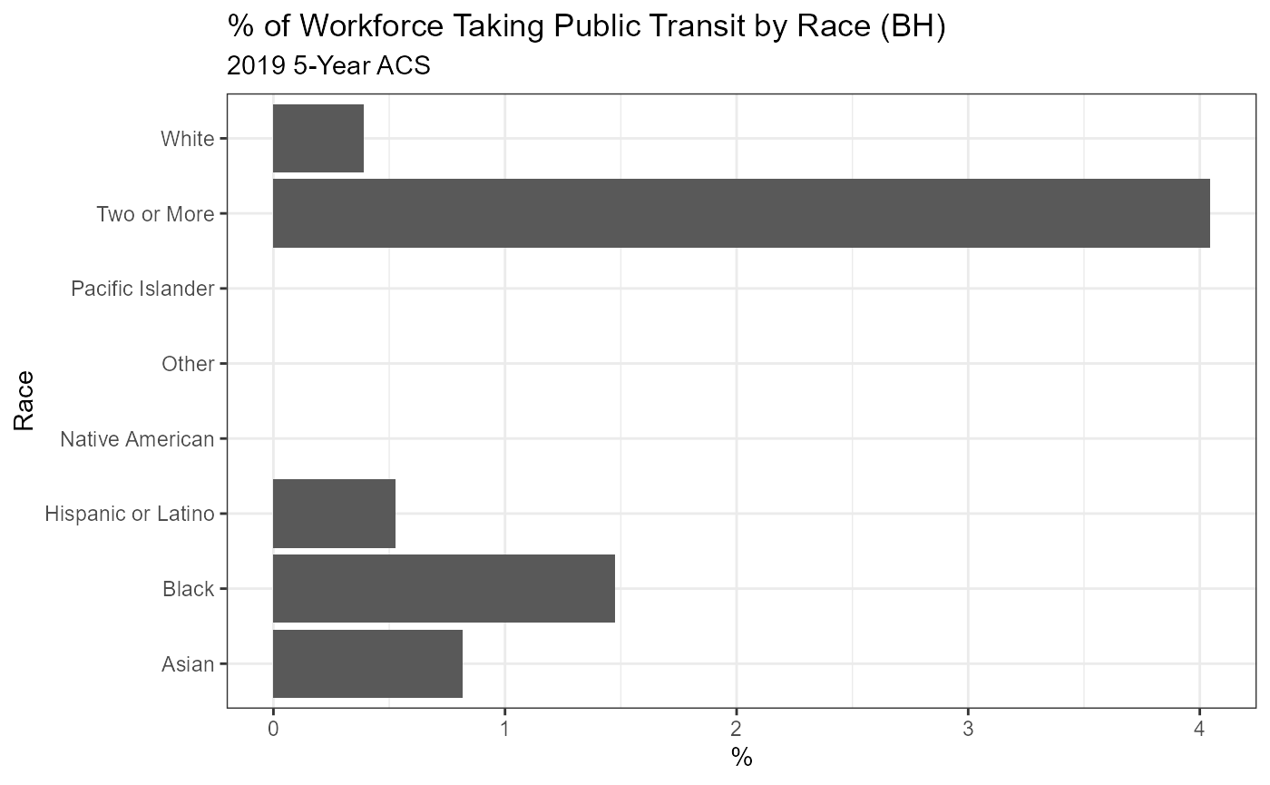
# PERCENT OF THE BLACK POPULATION IN BLACK HAWK USING EACH COMMUTE TYPE
blackHawkBlackAllCommutes <- blackHawkCombined  %>%
  filter(GEOID == 19013 & race == "Black")

ggplot(blackHawkBlackAllCommutes, aes(x = factor(variable), y = 100*percent_of_pop)) +
  geom_bar(stat = "identity") +
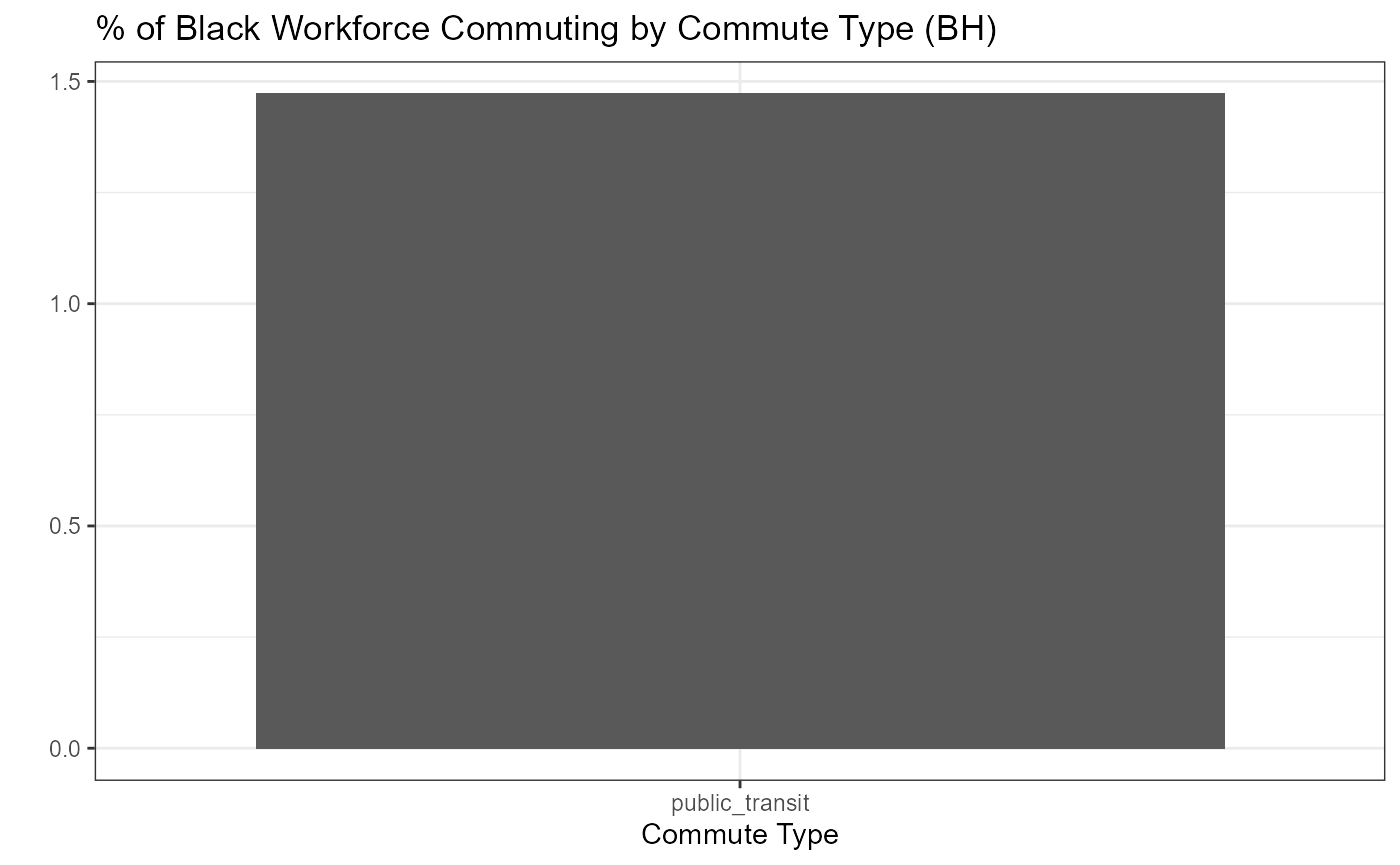
  labs(title = "% of Black Workforce Commuting by Commute Type (BH)", x = "Commute Type", y = "") +
  theme_bw()